Introduction to Convex Optimization Basic Concepts 详细

往期文章链接目录

Optimization problem

All optimization problems can be written as:

Optimization Categories

1. convex v.s. non-convex
   Deep Neural Network is non-convex

2. continuous v.s.discrete
   Most are continuous variable; tree structure is discrete

3. constrained v.s. non-constrained
   We add prior to make it a constrained problem

4. smooth v.s.non-smooth
   Most are smooth optimization

Different initialization brings different optimum (if not convex)

Idea: Give up global optimal and find a good local optimal.

• Purpose of pre-training: Find a good initialization to start training, and then find a better local optimal.

• Relaxation: Convert to a convex optimization problem.

• Brute force: If a problem is small, we can use brute force.

Affine sets

A set $C\subseteq {\mathbf{R}}^n$ is affine if the line through any two distinct points in $C$ lies in $C$, i.e., if for any $x1$, $x2\in C$ and $\theta \in \mathbf{R}$, we have $$\theta x_1+(1-\theta )x_2\in C.$$

Note: The line passing throught $x_1$ and $x_2$: $y=\theta x_1+(1-\theta )x_2$.

Affine combination

We refer to a point of the form ${\theta }_1{x}_1+{\theta }_2{x}_2+...+{\theta }_k{x}_k$, where ${\theta }_1+{\theta }_2+...+{\theta }_k=1$ as an affine combination of the points $x_1,x_2,...,x_k$. An affine set contains every affine combination of its points.

Affine hull

The set of all affine combinations of points in some set $C\subseteq {\mathbf{R}}^n$ is called the affine hull of $C$, and denoted $\mathbf{a}\mathbf{f}\mathbf{f}C$:

$$\mathbf{a}\mathbf{f}\mathbf{f}C=\{{\theta }_1{x}_1+{\theta }_2{x}_2+...+{\theta }_k{x}_k|x_1,x_2,...,x_k\in C,{\theta }_1+{\theta }_2+...+{\theta }_k=1\}.$$

The affine hull is the smallest affine set that contains $C$, in the following sense: if
$S$ is any affine set with $C\subseteq S$, then $\mathrm{aff}C\subseteq S$.

Affine dimension: We define the affine dimension of a set $C$ as the dimension of its affine hull.

Convex Sets

A set $C$ is convex if the line segment between any two points in $C$ lies in $C$, i.e., if for any $x1$, $x2\in C$ and any $\theta$ with $0\le \theta \le 1$, we have
$$\theta x_1+(1-\theta )x_2\in C.$$

Roughly speaking, a set is convex if every point in the set can be seen by every other
point. Every affine set is also convex, since it contains the entire line between any two distinct points in it, and therefore also the line segment between the points.

Convex combination

We call a point of the form ${\theta }_1{x}_1+{\theta }_2{x}_2+...+{\theta }_k{x}_k$, where ${\theta }_1+{\theta }_2+...+{\theta }_k=1$ and ${\theta }_i\ge 0,i=1,2,...k$, a convex combination of the points $x_1,...,x_k$.

Convex hull

The convex hull of a set $C$, denoted $\mathbf{c}\mathbf{o}\mathbf{n}\mathbf{v}C$, is the set of all convex combinations of points in $C$:

$$\mathbf{c}\mathbf{o}\mathbf{n}\mathbf{v}C=\{{\theta }_1{x}_1+{\theta }_2{x}_2+...+{\theta }_k{x}_k|x_i\in C,{\theta }_i\ge 0,i=1,...,k,{\theta }_1+{\theta }_2+...+{\theta }_k=1\}.$$

The convex hull $\mathrm{conv}C$ is always convex. It is the smallest convex set that contains $C$: If $B$ is any convex set that contains $C$, then $\mathrm{conv}C\subseteq B$.

Cones

A set $C$ is called a cone, or nonnegative homogeneous, if for every $x\in C$ and $\theta \ge 0$ we have $\theta x\in C$. A set $C$ is a convex cone if it is convex and a cone, which means that for any $x_1,x_2\in C$ and ${\theta }_1,{\theta }_2\ge 0$, we have

$${\theta }_1{x}_1+{\theta }_2{x}_2\in C$$

Hyperplanes and halfspaces

A hyperplane is a set of the form
$$\{x|a^{T}x=b\},$$

where $a\in {\mathbf{R}}^n,a\ne 0$, and $b\in \mathbf{R}$.

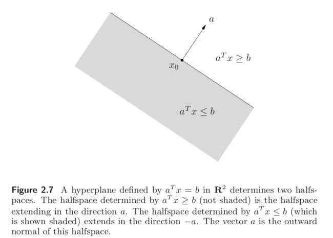
This geometric interpretation can be understood by expressing the hyperplane in the form

$$\{x|a^T(x-x_0)=0\},$$
where $x_0$ is any point in the hyperplane.

A hyperplane divides ${\mathbf{R}}^n$ into two halfspaces. A (closed) halfspace is a set of the form

$$\{x|a^{T}x\le b\}.$$

where $x_0\ne 0$. Halfspaces are convex but not affine. The set $ {x | a^T < b }$ is called an open halfspace.

Polyhedra

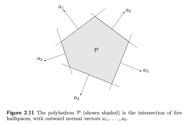
A polyhedron is defined as the solution set of a finite number of linear equalities and inequalities:

$$P=\{x|a_j^T\le b_j,j=1,...,m,c_j^{T}x=d_j,j=1,...,p\}$$

A polyhedron is thus the intersection of a finite number of halfspaces and hyperplanes. Here is the compact notations:

$$P=\{x|Ax⪯b,Cx=d\}$$

Linearly Independent v.s. Affinely Independent

Consider the vectors (1,0), (0,1) and (1,1). These are affinely independent, but not independent. If you remove any one of them, their affine hull has dimension one. In contrast, the span of any two of them is all of ${\mathbf{R}}^2$, and hence these are not independent.

Simplexes

Suppose the $k+1$ points $v_0,...,v_k\in {\mathbf{R}}^n$ are affinely independent, which means $v_1-v_0,...,v_k-v_0$ are linearly independent. The simplex determined by them is given by

$$C=\mathbf{c}\mathbf{o}\mathbf{n}\mathbf{v}\{v_0,...,v_k\}=\{{\theta }_0{v}_0+...+{\theta }_k{v}_k|\theta ⪰0,1^T\theta =1\}$$

Note:

• The affine dimension of this simplex is $k$.

A 1-dimensional simplex is a line segment; a 2-dimensional simplex is a triangle (including its interior); and a 3-dimensional simplex is a tetrahedron.

What is the key distinction between a convex hull and a simplex?

If the elements of the set on which the convex hull is defined are affinely independent, then the convex hull and the simplex defined on this set are the same. Otherwise, simplex can’t be defined on this set, but convex hull can.

Convex Functions

• A function $f:{\mathbf{R}}^n\to \mathbf{R}$ is convex if dom $f$ is a convex set and if for all $x$, $y\in \mathbf{d}\mathbf{o}\mathbf{m}f$, and $\theta$ with $ 0 \leq \theta \leq 1$, we have

$$f(\theta x+(1-\theta )y)\le \theta f(x)+(1-\theta )f(y).$$

• We say $f$ is concave is $-f$ is convex, and strictly concave if $-f$ is strictly convex.

• A function is convex if and only if it is convex when restricted to any line that intersects its domain. In other words f is convex if and only if for all $x\in \mathbf{d}\mathbf{o}\mathbf{m}f$ and all $v$, the function $g(t)=f(x+tv)$ is convex (on its domain, $\{t|x+tv\in \mathbf{d}\mathbf{o}\mathbf{m}f\}$).

First-order conditions

• Suppose $f$ is differentiable, then $f$ is convex if and only if $\mathbf{d}\mathbf{o}\mathbf{m}f$ is convex and
  $$f(y)\ge f(x)+\nabla f(x{)}^T(y-x)$$ holds for all $x,y\in \mathbf{d}\mathbf{o}\mathbf{m}f$

• For a convex function, the first-order Taylor approximation is in fact a global underestimator of the function. Conversely, if the first-order Taylor approximation of a function is always a global underestimator of the function, then the function is convex.

• The inequality shows that from local information about a convex function (i.e., its value and derivative at a point) we can derive global information (i.e., a global underestimator of it).

Second-order conditions

• Suppose that $f$ is twice differentiable. The $f$ is convex if and only if $\mathbf{d}\mathbf{o}\mathbf{m}f$ is convex and its Hessian is positive semidefinite: for all $x\in \mathbf{d}\mathbf{o}\mathbf{m}f$,
  $${\nabla }^{2}f(x)⪰0.$$

• $f$ is concave if and only if $\mathbf{d}\mathbf{o}\mathbf{m}f$ is convex and ${\nabla }^{2}f(x)⪯0$ for all $x\in \mathbf{d}\mathbf{o}\mathbf{m}f$.

• If $ \nabla^2f(x) \succ 0$ for all $x\in \mathbf{d}\mathbf{o}\mathbf{m}f$, then $f$ is strictly convex. The converse is not true. e.x. $f(x)=x^4$ has zero second derivative at $x=0$ but is strictly convex.

• Quadratic functions: Consider the quadratic function $f:{\mathbf{R}}^n\to \mathbf{R}$, with $\mathbf{d}\mathbf{o}\mathbf{m}f={\mathbf{R}}^n$, given by
  $$f(x)=(1/2)x^{T}Px+q^{T}x+r,$$
  with $P\in {\mathbf{S}}^n,q\in {\mathbf{R}}^n$, and $r\in \mathbf{R}$. Since ${\nabla }^{2}f(x)=P$ for all x, f is convex if and only if $P⪰0$ (and concave if and only if $P⪯0$).

Examples of Convex and Concave Functions

• Exponential. $e^{ax}$ is convex on $\mathbf{R}$, for any $a\in \mathbf{R}$.

• Powers. $x^a$ is convex on ${\mathbf{R}}_{++}$ when $a\ge 1$ or $a\le 0$, and concave for $0\le a\le 1$.

• Powers of absolute value. $|x{|}^p$, for $p\ge 1$, is convex on $\mathbf{R}$.

• Logarithm. $logx$ is concave on $R_{++}$.

• Negative Entropy. $xlogx$ (either on ${\mathbf{R}}_{++}$, or on ${\mathbf{R}}_{+}$, defined as $0$ for $x=0$) is convex.

• Norms. Every norm on ${\mathbf{R}}^n$ is convex.

• Max function. $f(x)=max\{x_1,...,x_n\}$ is convex on ${\mathbf{R}}^n$.

• Quadratic-over-linear function. The function $f(x,y)=x^2/y$, with
  $$\mathbf{d}\mathbf{o}\mathbf{m}f=\mathbf{R}\times {\mathbf{R}}_{++}=\{(x,y)\in {\mathbf{R}}^2|y>0\},$$ is convex.

• Log-sum-exp. The function $f(x)=log(e^{x_1}+\cdot \cdot \cdot +e^{x_n})$ is convex on ${\mathbf{R}}^n$.

• Geometric mean. The geometric mean $f(x)=({\prod }_{i=1}^n{x}_i{)}^{1/n}$ is concave on $\mathbf{d}\mathbf{o}\mathbf{m}f={\mathbf{S}}_{++}^n$

• Log-determinant. The function $f(X)=\mathrm{l}\mathrm{o}\mathrm{g}\mathrm{d}\mathrm{e}\mathrm{t}X$ is concave.

---

Reference: Convex Optimization by Stephen Boyd and Lieven Vandenberghe.

往期文章链接目录