局部异常因子与KL散度异常检测算法简述
Local Outlier Factor
Given local outlier factors, we can detect the outliers that are always away from most of the samples. In order to outline the algorithm, some concepts must go first:
Reachability Distance
where x(k) stands for the k th point nearest to x in training set {xi}ni=1 . Note that k is manually selected.
Local Reachability Density
Local Outlier Factor
Evidently, as the LOF of x ascends, the probability that x is an outlier also goes up. Theoretically, it is an easy algorithm with intuitive principle. However, when n is a very large number, it also requires tremendous computation amount.
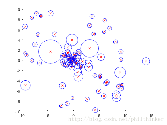
Here is a simple example
n=100; x=[(rand(n/2,2)-0.5)*20; randn(n/2,2)]; x(n,1)=14;
k=3; x2=sum(x.^2,2);
[s, t]=sort(sqrt(repmat(x2,1,n)+repmat(x2',n,1)-2*x*x'), 2);

for i=1:k+1
    for j=1:k
        RD(:,j)=max(s(t(t(:,i),j+1),k), s(t(:,i),j+1));
    end
    LRD(:,i)=1./mean(RD,2);
end
LOF=mean(LRD(:,2:k+1),2)./LRD(:,1);

figure(1); clf; hold on
plot(x(:,1),x(:,2),'rx');
for i=1:n
    plot(x(i,1),x(i,2),'bo', 'MarkerSize', LOF(i)*10);
end
KL Divergence
In unsupervised learning problems, there is usually little information about the outliers. However, when some known normal sample set {x′i′}n′i′=1 is given, we may be confident to figure out the outliers in the test set {xi}ni=1 to some degree.
Kullback-Leibler (KL) divergence, also known as Relative Entropy, is a powerful tool to estimate the probability density ratio of normal samples to test samples-
where p′(x) is the probability density of normal samples and p(x) is that of test ones, and avoid direct calculation of the ratio. The ratio of normal sample approaches 1 but of an outlier is away from 1.
To begin with, let transform the model of density ratio to a parameterized linear model:
where α=(α1,⋯,αb)T is the parameter vector and ψ(x)=(ψ1,⋯,ψb)T is a non-negative basis function vector. Then wα(x)p(x) can be seen as an estimation of p′(x) . Define the similarity between wα(x)p(x) and p′(x) as KL distance, i.e.
In general case, KL distance is non-negative and equals to zero only if wαp=p′ . When KL distance is considerably small, wαp can be regarded near to p′ . In order to guarantee that wαp is well-defined, we apply the following constraint
Then by approximation, we can transform the estimation above to the following optimal problem:
We briefly summarize the estimation process:
- Initialize α .
- Repeatedly carry out the following process until α comes a suitable precision:
- α←α+ϵAT(1./Aα)
- α←α+(1−bTα)b(bTb)
- α←max(0,α)
- α←α/(bTα)
where A is the matrix whose (i′,j) th element is ψj(x′i′) . b is the vector whose j th element is 1n∑ni=1ψj(xi) .
Here is an example (Gaussian Kernal Model):
function [ a ] = KLIEP( k, r )

a0=rand(size(k,2),1); b=mean(r)'; c=sum(b.^2);
for o=1:1000
    a=a0+0.01*k'*(1./k*a0); a=a+b*(1-sum(b.*a))/c;
    a=max(0,a); a=a/sum(b.*a);
    if norm(a-a0)<0.001, break, end
    a0=a;
end

endn=100; x=randn(n,1); y=randn(n,1); y(n)=5;
hhs=2*[1,5,10].^2; m=5;
x2=x.^2; xx=repmat(x2,1,n)+repmat(x2',n,1)-2*(x*x');
y2=y.^2; yx=repmat(y2,1,n)+repmat(x2',n,1)-2*y*x';
u=floor(m*(0:n-1)/n)+1;
u=u(randperm(n));
for hk=1:length(hhs)
hh=hhs(hk);k=exp(-xx/hh); r=exp(-yx/hh);
for i=1:m
g(hk,i)=mean(k(u==i,:)*KLIEP(k(u~=i,:),r));
end
end
[gh,ggh]=max(mean(g,2));
HH=hhs(ggh);
k=exp(-xx/HH); r=exp(-yx/HH); s=r*KLIEP(k,r);
figure(1); clf; hold on; plot(y,s,'rx');SVM
Furthermore, outlier detection can be done using support vector machine techniques. Due to the time limit, we just outline the main structure of that algorithm.
A typical SVM outlier detector gives a hyper-ball that contains nearly all the sample points. Then a point which is outlying the hyper-ball can be seen as an outlier. Concretely speaking, we get the center c and radius R by solving the following optimal problem:
It can be solved by using Lagrange multiplers:
Then its dual problem can be formulated as:
KKT condition:
Therefore, the dual problem can be solved by
It is in the form of typical quadratic programming problem. After solving it, we are able to further solve c and R :
where xi is the support vector satisfying ∥xi−c∥2=R2 and 0<αi<C .
Hence, when a sample point x satisfies
it can be viewed as an outlier.

