图卷积网络GRAPH CONVOLUTIONAL NETWORKS

GRAPH CONVOLUTIONAL NETWORKS

THOMAS KIPF, 30 SEPTEMBER 2016https://tkipf.github.io/graph-convolutional-networks/

带一阶滤波器的多层图卷积网络

Overview 

综述

Many important real-world datasets come in the form of graphs or networks: social networks, knowledge graphs, protein-interaction networks, the World Wide Web, etc. (just to name a few). Yet, until recently, very little attention has been devoted to the generalization of neural network models to such structured datasets.

许多重要的现实世界数据集以图表或网络的形式出现:社交网络、知识图谱、蛋白质交互网络、万维网等等(仅举几例)。然而，直到最近，很少有人关注神经网络模型泛化到这样的图表、网络形式的结构化数据集。

In the last couple of years, a number of papers re-visited this problem of generalizing neural networks to work on arbitrarily structured graphs (Bruna et al., ICLR 2014; Henaff et al., 2015; Duvenaud et al., NIPS 2015; Li et al., ICLR 2016; Defferrard et al., NIPS 2016; Kipf & Welling, ICLR 2017), some of them now achieving very promising results in domains that have previously been dominated by, e.g., kernel-based methods, graph-based regularization techniques and others.

在过去的几年里，大量论文重新讨论了将神经网络推广到任意结构图上的问题(Bruna et al., ICLR 2014; Henaff et al., 2015; Duvenaud et al., NIPS 2015; Li et al., ICLR 2016; Defferrard et al., NIPS 2016; Kipf & Welling, ICLR 2017), 其中基于核函数的方法、基于图的正则化技术等已经在不同领域中取得了非常有前途的结果。

In this post, I will give a brief overview of recent developments in this field and point out strengths and drawbacks of various approaches. The discussion here will mainly focus on two recent papers:

在这篇文章中，我将简要概述这一领域的最新发展，并指出各种方法的优缺点。这里的讨论主要集中在最近的两篇论文上

• Kipf & Welling (ICLR 2017), Semi-Supervised Classification with Graph Convolutional Networks (disclaimer: I'm the first author)图卷积网络的半监督分类(声明:我是第一作者)
• Defferrard et al. (NIPS 2016), Convolutional Neural Networks on Graphs with Fast Localized Spectral Filtering图上的卷积神经网络具有快速的局部谱滤波

and a review/discussion post by Ferenc Huszar: How powerful are Graph Convolutions? that discusses some limitations of these kinds of models. I wrote a short comment on Ferenc's review here (at the very end of this post).

Ferenc Huszar的综述/讨论:图卷积有多强大？讨论了这类模型的一些局限性。我在这里(在这篇文章的最后)对Ferenc的综述写了一个简短的评论。

Outline大纲

• Short introduction to neural network models on graphs简要介绍图的神经网络模型
• Spectral graph convolutions and Graph Convolutional Networks (GCNs)谱图卷积和图卷积网络
• Demo: Graph embeddings with a simple 1st-order GCN model案例:图形嵌入与一个简单的一阶GCN模型
• GCNs as differentiable generalization of the Weisfeiler-Lehman algorithmGCNs作为weisfeler - lehman算法的可微推广

If you're already familiar with GCNs and related methods, you might want to jump directly to Embedding the karate club network.如果您已经熟悉GCNs和相关的方法，您可能想要直接跳到Embedding the karate club network。

How powerful are Graph Convolutional Networks?

图卷积网络有多强大?

Recent literature相关文献

Generalizing well-established neural models like RNNs or CNNs to work on arbitrarily structured graphs is a challenging problem. Some recent papers introduce problem-specific specialized architectures (e.g. Duvenaud et al., NIPS 2015; Li et al., ICLR 2016; Jain et al., CVPR 2016), others make use of graph convolutions known from spectral graph theory1 (Bruna et al., ICLR 2014; Henaff et al., 2015) to define parameterized filters that are used in a multi-layer neural network model, akin to "classical" CNNs that we know and love.

推广成熟的神经模型例如RNN或CNN用于任意结构图表是个有挑战性的问题。最近的一些论文，介绍了针对特定问题的架构（e.g. Duvenaud et al., NIPS 2015; Li et al., ICLR 2016; Jain et al., CVPR 2016），还有一些利用谱图理论（Bruna et al., ICLR 2014; Henaff et al., 2015）的图卷积来定义用于多层神经网络模型的参数化滤波器，类似我们熟悉的“经典”CNN。

More recent work focuses on bridging the gap between fast heuristics and the slow2, but somewhat more principled, spectral approach. Defferrard et al. (NIPS 2016) approximate smooth filters in the spectral domain using Chebyshev polynomials with free parameters that are learned in a neural network-like model. They achieve convincing results on regular domains (like MNIST), closely approaching those of a simple 2D CNN model.

最近的工作重点是弥合快速启发式和缓慢启发式之间的差距2、但更有规则性的谱分方法间的差距。Defferrard 等人（NIPS 2016）用神经网络模型学习的自由参数的Chebyshev多项式模拟了谱域的平滑滤波。他们在正则区域（像是MNIST）得到了有说服力的结果，很接近简单2D CNN模型的结果。

In Kipf & Welling (ICLR 2017), we take a somewhat similar approach and start from the framework of spectral graph convolutions, yet introduce simplifications (we will get to those later in the post) that in many cases allow both for significantly faster training times and higher predictive accuracy, reaching state-of-the-art classification results on a number of benchmark graph datasets.

Kipf & Welling （2016）的研究采用了类似的方法，从图谱卷积框架开始，介绍了许多情况下能同时显著加快训练时间和提高预测准确度的最简化方法，在许多基准图集上得到了极好的分类结果。

GCNs Part I: Definitions

GCNS 第一部分：定义

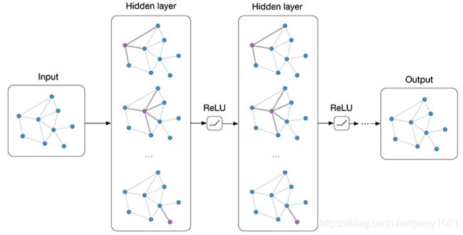
Currently, most graph neural network models have a somewhat universal architecture in common. I will refer to these models as Graph Convolutional Networks (GCNs); convolutional, because filter parameters are typically shared over all locations in the graph (or a subset thereof as in Duvenaud et al., NIPS 2015).

目前，大多数图神经网络模型都有一个某种程度上通用的普遍框架。我把这些模型称作图卷积网络（Graph Convolutional Networks, GCNs）；卷积，是因为滤波器参数通常在图的所有位置中共享（或在其子集，参见 Duvenaud et al. NIPS 2015）。

For these models, the goal is then to learn a function of signals/features on a graph G=(V,E)which takes as input:

对这些模型来说，目标是学习图的信号/特征函数G =（V, E），它的输入如下：

• A feature description xi for every node i; summarized in a N×D feature matrix X (N: number of nodes, D: number of input features)对每个节点 i 的特征描述为 xi；概括在特征矩阵 N×D（N：节点数，D：输入特征数)
• A representative description of the graph structure in matrix form; typically in the form of an adjacency matrix A (or some function thereof)矩阵形式的图结构的典型描述，通常以邻接矩阵A(或其某个函数)的形式出现

and produces a node-level output Z (an N×F feature matrix, where F is the number of output features per node). Graph-level outputs can be modeled by introducing some form of pooling operation (see, e.g. Duvenaud et al., NIPS 2015).并产生节点级输出Z（N×F 特征矩阵，F是每个节点输出特征的数量）。图层面的输出可以引入某些池化操作（参见：e.g. Duvenaud et al., NIPS 2015）。

Every neural network layer can then be written as a non-linear function：

每个神经网络层可以写成一个非线性函数：

H(l+1)=f(H(l),A),

with H(0)=X and H(L)=Z(or z for graph-level outputs), L being the number of layers. The specific models then differ only in how f(⋅,⋅)is chosen and parameterized.

H(0) = X 和 H(L) = Z （或在图层面的输出时，z），L表示层数。模型不同的只有怎样选择 f(⋅,⋅)的参数设定。

GCNs Part II: A simple example

GCNs 第二部分：一个简单的例子

As an example, let's consider the following very simple form of a layer-wise propagation rule:

举个例子，让我们看下面这个十分简单的分层优化传播规律：

f(H(l),A)=σ(AH(l)，W(l)),

where W(l) is a weight matrix for the ll-th neural network layer and σ(⋅)σ(⋅) is a non-linear activation function like the ReLU. Despite its simplicity this model is already quite powerful (we'll come to that in a moment).

W(l) 是神经网络 l 层的权重矩阵，σ(⋅)是像ReLU这样的非线性激活函数。虽然这个模型非常简单，但它已经是非常强大的(我们一会儿会讲到这一点)。

But first, let us address two limitations of this simple model: multiplication with A means that, for every node, we sum up all the feature vectors of all neighboring nodes but not the node itself (unless there are self-loops in the graph). We can "fix" this by enforcing self-loops in the graph: we simply add the identity matrix to A.

但让我们先了解这个简单模型的两点局限性：
1.与 A 相乘意味着对每个节点，我们需要把所有相邻节点的所有特征矢量相加，但不能加上节点本身（除非图上有自回路）。我们可以强迫图执行自回路：在单位矩阵中加上A。

The second major limitation is that A is typically not normalized and therefore the multiplication with A will completely change the scale of the feature vectors (we can understand that by looking at the eigenvalues of A). Normalizing A such that all rows sum to one, i.e. D−1A, where D is the diagonal node degree matrix, gets rid of this problem. Multiplying with D−1A now corresponds to taking the average of neighboring node features.

2.第二个局限性主要是 A 通常不是归一化的，因此与 A 相乘将完全改变特征向量的分布范围（我们可以通过查看 A 的特征值来理解）。归一化 A 使得所有行总和为 1，即 D^-1 A，其中 D 是对角节点度矩阵，这样即可避免这个问题。归一化后，乘以 D^-1 A 相当于取相邻节点特征的平均值。

In practice, dynamics get more interesting when we use a symmetric normalization, i.e.  D^-1/2 A D^-1/2(as this no longer amounts to mere averaging of neighboring nodes). Combining these two tricks, we essentially arrive at the propagation rule introduced in Kipf & Welling (ICLR 2017):

在实际应用中可使用对称归一化，如 D^-1/2 A D^-1/2（不仅仅是相邻节点的平均），模型动态会变得更有趣。结合这两个技巧，我们基本上获得了Kipf & Welling (ICLR 2017)文章中介绍的传播规则：

with A^=A+I, where I is the identity matrix and D^is the diagonal node degree matrix of A^.

式中 A^ =A+I，I 是单位矩阵，D 是 A 的对角节点度矩阵。。

In the next section, we will take a closer look at how this type of model operates on a very simple example graph: Zachary's karate club network (make sure to check out the Wikipedia article!).

在下一节中，我们将仔细研究这种类型的模型如何在一个非常简单的示例图上运行：Zachary's karate club network   Zachary的空手道俱乐部网络（make sure to check out the Wikipedia article!)）。

GCNs Part III: Embedding the karate club network

GCNs 第三部分： 嵌入空手道俱乐部网络

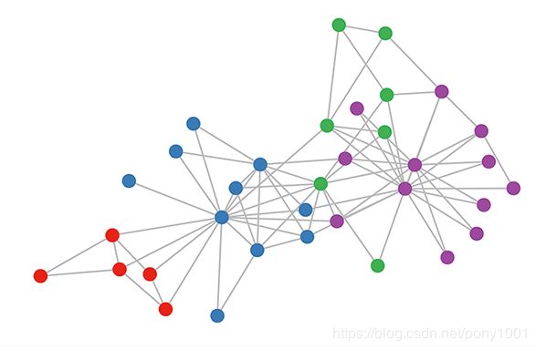
Karate club graph, colors denote communities obtained via modularity-based clustering (Brandes et al., 2008).

空手道俱乐部图，颜色表示通过基于模块化的聚类获得的 communities社区(Brandes et al., 2008).

Let's take a look at how our simple GCN model (see previous section or Kipf & Welling, ICLR 2017) works on a well-known graph dataset: Zachary's karate club network (see Figure above).让我们来看看我们简单的GCN模型（参见上一节或Kipf & Welling, ICLR 2017）如何在著名的图形数据集上工作：Zachary的空手道俱乐部网络（见上图）。

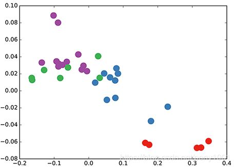
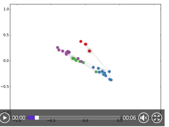
We take a 3-layer GCN with randomly initialized weights. Now, even before training the weights, we simply insert the adjacency matrix of the graph and X=I (i.e. the identity matrix, as we don't have any node features) into the model. The 3-layer GCN now performs three propagation steps during the forward pass and effectively convolves the 3rd-order neighborhood of every node (all nodes up to 3 "hops" away). Remarkably, the model produces an embedding of these nodes that closely resembles the community-structure of the graph (see Figure below). Remember that we have initialized the weights completely at random and have not yet performed any training updates (so far)!
我们取一个3层的GCN，它的权值是随机初始化的。现在，甚至在训练权值之前，我们只需插入图的邻接矩阵以及X=I (例如，单位矩阵，因为我们没有任何特征）插入到模型。3层GCN现在前向传播期间执行三个传播步骤，并有效地卷积每个节点（图的节点）的3阶邻域（所有节点最多3“跳”）。值得注意的是，该模型生成了这些节点的嵌入，它们与图中的社区结构非常相似(见下图)。请记住，我们已经完全随机地初始化了权值，并且还没有执行任何训练更新(到目前为止)!

GCN embedding (with random weights) for nodes in the karate club network.

在空手道俱乐部网络的节点中嵌入GCN(随机权值)。

This might seem somewhat surprising. A recent paper on a model called DeepWalk (Perozzi et al., KDD 2014) showed that they can learn a very similar embedding in a complicated unsupervised training procedure. How is it possible to get such an embedding more or less "for free" using our simple untrained GCN model?

这似乎有点令人惊讶。最近一篇关于DeepWalk模型的论文(Perozzi et al.， KDD 2014)表明，他们可以在复杂的无监督训练过程中得到相似的嵌入。那我们怎么可能仅仅使用未经训练的简单 GCN 模型，就得到这样的嵌入呢？

We can shed some light on this by interpreting the GCN model as a generalized, differentiable version of the well-known Weisfeiler-Lehman algorithm on graphs. The (1-dimensional) Weisfeiler-Lehman algorithm works as follows3:

通过将GCN模型解释为众所周知的图上的weisfeler - lehman算法的广义可微版本，我们可以对此提供一些启发。

For all nodes vi∈G:对所有的节点vi∈G:

• Get features4 {hvj}of neighboring nodes {vj}
• 对所有的节点 vi∈G   求解邻近节点 {vj} 的特征 {hvj}
• Update node feature hvi←hash(∑jhvj), where hash(⋅) is (ideally) an injective hash function
• 通过 hvi←hash（Σj hvj） 更新节点特征，该式中 hash（理想情况下）是一个单射散列函数
• Repeat for k steps or until convergence.重复k个步骤，直到收敛。

In practice, the Weisfeiler-Lehman algorithm assigns a unique set of features for most graphs. This means that every node is assigned a feature that uniquely describes its role in the graph. Exceptions are highly regular graphs like grids, chains, etc. For most irregular graphs, this feature assignment can be used as a check for graph isomorphism (i.e. whether two graphs are identical, up to a permutation of the nodes).

在实际应用中，Weisfeiler-Lehman 算法可以为大多数图赋予一组独特的特征。这意味着每个节点都被分配了一个独一无二的特征，该特征描述了该节点在图中的作用。但这对于像网格、链等高度规则的图是不适用的。对大多数不规则的图而言，特征分配可用于检查图的同构（即从节点排列，看两个图是否相同）。

Going back to our Graph Convolutional layer-wise propagation rule (now in vector form):

回到我们图卷积的层传播规则（以向量形式表示）：

where j indexes the neighboring nodes of vi. cij is a normalization constant for the edge (vi,vj) which originates from using the symmetrically normalized adjacency matrix D-1/2 A D-1/2  in our GCN model.

式中，j 表示 vi 的相邻节点。cij 是使用我们的 GCN 模型中的对称归一化邻接矩阵 D-1/2 A D-1/2 生成的边 （v_i，v_j） 的归一化常数。

We now see that this propagation rule can be interpreted as a differentiable and parameterized (with W(l)) variant of the hash function used in the original Weisfeiler-Lehman algorithm. If we now choose an appropriate non-linearity and initialize the random weight matrix such that it is orthogonal (or e.g. using the initialization from Glorot & Bengio, AISTATS 2010), this update rule becomes stable in practice (also thanks to the normalization with cijcij). And we make the remarkable observation that we get meaningful smooth embeddings where we can interpret distance as (dis-)similarity of local graph structures!

我们可以将该传播规则解释为在原始的 Weisfeiler-Lehman 算法中使用的 hash 函数的可微和参数化（对 W（l））变体。如果我们现在选择一个适当的、非线性的的矩阵，并且初始化其随机权重，使它是正交的，（或者使用 Glorot & Bengio, AISTATS 2010 提出的初始化）那么这个更新规则在实际应用中会变得稳定（这也归功于归一化中的 c_ij 的使用）。我们得出了很有见地的结论，即我们得到了一个很有意义的平滑嵌入，其中可以用距离远近表示局部图结构的相似性/不相似性！

GCNs Part IV: Semi-supervised learning

GCNs 第4部分：半监督学习

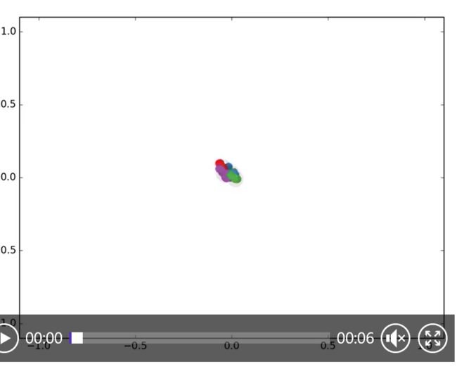
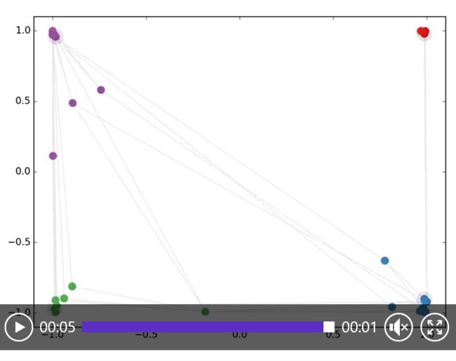
Since everything in our model is differentiable and parameterized, we can add some labels, train the model and observe how the embeddings react. We can use the semi-supervised learning algorithm for GCNs introduced in Kipf & Welling (ICLR 2017). We simply label one node per class/community (highlighted nodes in the video below) and start training for a couple of iterations5:

由于我们模型中的所有内容都是可微分且参数化的，因此可以添加一些标签，使用这些标签训练模型并观察嵌入如何反应。我们可以使用Kipf & Welling (ICLR 2017).文章中介绍的 GCN 的半监督学习算法。我们只需对每类/共同体（下面视频中突出显示的节点）的一个节点进行标记，然后开始进行几次迭代训练：

Semi-supervised classification with GCNs: Latent space dynamics for 300 training iterations with a single label per class. Labeled nodes are highlighted.

用 GCNs 进行半监督分类：对每类仅仅标记一个标签，（突出显示标记节点）进行 300 次迭代训练得到隐空间的动态。

Note that the model directly produces a 2-dimensional latent space which we can immediately visualize. We observe that the 3-layer GCN model manages to linearly separate the communities, given only one labeled example per class. This is a somewhat remarkable result, given that the model received no feature description of the nodes. At the same time, initial node features could be provided, which is exactly what we do in the experiments described in our paper (Kipf & Welling, ICLR 2017) to achieve state-of-the-art classification results on a number of graph datasets.

注意，该模型直接产生了一个二维的潜在空间，我们可以直接可视化。我们观察到，3层的GCN模型能够线性地分离社区，每个类只给出一个标记的示例。考虑到模型没有收到节点的特征描述，这是一个有点值得注意的结果。同时，可以提供初始节点特征，这正是我们在本文中所做的实验(Kipf & Welling, ICLR 2017) 在许多图形数据集上实现最新的分类结果。

Conclusion结论

Research on this topic is just getting started. The past several months have seen exciting developments, but we have probably only scratched the surface of these types of models so far. It remains to be seen how neural networks on graphs can be further taylored to specific types of problems, like, e.g., learning on directed or relational graphs, and how one can use learned graph embeddings for further tasks down the line, etc. This list is by no means exhaustive and I expect further interesting applications and extensions to pop up in the near future. Let me know in the comments below if you have some exciting ideas or questions to share!

有关这个领域的研究才刚刚起步。在过去的几个月中，该领域已经获得了振奋人心的发展，但是迄今为止，我们可能只是抓住了这些模型的表象。而神经网络如何在图论上针对特定类型的问题进行研究，如在定向图或关系图上进行学习，以及如何使用学习的图嵌入来完成下一步的任务等问题，还有待进一步探索。本文涉及的内容绝非详尽无遗的，而我希望在不久的将来会有更多有趣的应用和扩展。

 

本译文参考了：https://www.cnblogs.com/ranup/p/10914494.html