Matlab自适应滤波器设计Demo——LMS,RLS
以下是从Matlab的帮助文档里摘来的滤波器Demo。
滤波器、均衡器,我就不多说了。
前面有系列文章,滤波器的设计。如LMS滤波器、经典FIR滤波器等。
这里直接使用Matlab的工具箱。
Choose an Adaptive Algorithm. Configuring an equalizer involves choosing an adaptive algorithm and indicating your choice when creating an equalizer object in the MATLAB environment.
Although the best choice of adaptive algorithm might depend on your individual situation, here are some generalizations that might influence your choice:
The LMS algorithm executes quickly but converges slowly, and its complexity grows linearly with the number of weights.
The RLS algorithm converges quickly, but its complexity grows with the square of the number of weights, roughly speaking. This algorithm can also be unstable when the number of weights is large.
The various types of signed LMS algorithms simplify hardware implementation.
The normalized LMS and variable-step-size LMS algorithms are more robust to variability of the input signal's statistics (such as power).
The constant modulus algorithm is useful when no training signal is available, andworks best for constant modulus modulationssuch as PSK.
However, if CMA has no additional side information, it can introduce phase ambiguity. For example, CMA might find weights that produce a perfect QPSK constellation but might introduce a phase rotation of 90, 180, or 270 degrees. Alternatively, differential modulation can be used to avoid phase ambiguity.
基本步骤
% Build a set of test data.
hMod = comm.BPSKModulator; % BPSKModulator System object
x = step(hMod,randi([0 1],1000,1)); % BPSK symbols
rxsig = conv(x,[1 0.8 0.3]);  % Received signal
% Create an equalizer object.
eqlms = lineareq(8,lms(0.03));
% Change the reference tap index in the equalizer.
eqlms.RefTap = 4;
% Apply the equalizer object to a signal.
y = equalize(eqlms,rxsig,x(1:200));
In this example, eqlms is an equalizer object that describes a linear LMS equalizer having eight weights and a step size of 0.03. At first, the reference tap index in the equalizer has a default value, but assigning a new value to the property eqlms.RefTap changes this index. Finally, the equalize command uses the eqlms object to equalize the signal rxsig using the training sequence x(1:200).
恒定步长LMS
% The following code illustrates how to use
% equalize with a training sequence.
% The training sequence in this case is just
% the beginning of the transmitted message.

% Set up parameters and signals.
M = 4; % Alphabet size for modulation
msg = randi([0 M-1],1500,1); % Random message
hMod = comm.QPSKModulator('PhaseOffset',0);
modmsg = step(hMod,msg); % Modulate using QPSK.
trainlen = 500; % Length of training sequence
chan = [.986; .845; .237; .123+.31i]; % Channel coefficients
filtmsg = filter(chan,1,modmsg); % Introduce channel distortion.

% Equalize the received signal.
eq1 = lineareq(8, lms(0.01)); % Create an equalizer object. % 8 taps,lms算法,步长0.01
eq1.SigConst = step(hMod,(0:M-1)')'; % Set signal constellation. % 标准星座图
[symbolest,yd] = equalize(eq1,filtmsg,modmsg(1:trainlen)); % Equalize. % 均衡器obj,需要均衡的信号,训练序列

% Plot signals.
h = scatterplot(filtmsg,1,trainlen,'bx'); hold on;
scatterplot(symbolest,1,trainlen,'g.',h);
scatterplot(eq1.SigConst,1,0,'k*',h);
legend('Filtered signal','Equalized signal',...
   'Ideal signal constellation');
hold off;

% Compute error rates with and without equalization.
hDemod = comm.QPSKDemodulator('PhaseOffset',0);
demodmsg_noeq = step(hDemod,filtmsg); % Demodulate unequalized signal.
demodmsg = step(hDemod,yd); % Demodulate detected signal from equalizer.
hErrorCalc = comm.ErrorRate; % ErrorRate calculator
ser_noEq = step(hErrorCalc, ...
    msg(trainlen+1:end), demodmsg_noeq(trainlen+1:end));
reset(hErrorCalc)
ser_Eq = step(hErrorCalc, msg(trainlen+1:end),demodmsg(trainlen+1:end));
disp('Symbol error rates with and without equalizer:')
disp([ser_Eq(1) ser_noEq(1)])
eq1 =
EqType: 'Linear Equalizer'
AlgType: 'LMS'
nWeights: 8
nSampPerSym: 1
RefTap: 1
SigConst: [1x4 double]
StepSize: 0.0100
LeakageFactor: 1
Weights: [1x8 double]
WeightInputs: [1x8 double]
ResetBeforeFiltering: 1
NumSamplesProcessed: 1500
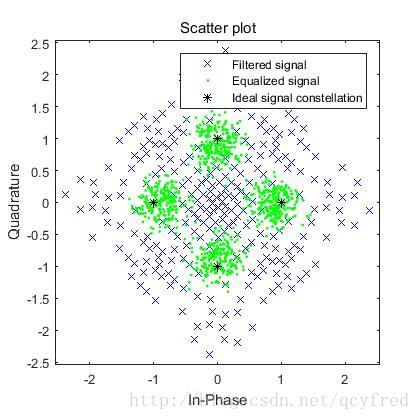
The example goes on to determine how many errors occur in trying to recover the modulated message with and without the equalizer. The symbol error rates, below, show that the equalizer improves the performance significantly.
Symbol error rates with and without equalizer:
         0    0.3410
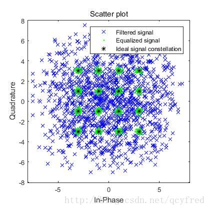
The example also creates a scatter plot that shows the signal before and after equalization, as well as the signal constellation for QPSK modulation. Notice on the plot that the points of the equalized signal are clustered more closely around the points of the signal constellation.
RLS算法
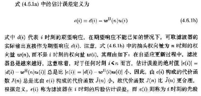
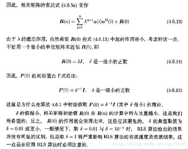
原理摘自于张贤达的《现代信号处理》,清华大学出版社。
省去了一些,放了一些基本思想上来。完整过程请自行阅读有关内容。
The rls function creates an adaptive algorithm object that you can use with the lineareq function or dfe function to create an equalizer object. You can then use the equalizer object with theequalize function to equalize a signal. To learn more about the process for equalizing a signal, see Adaptive Algorithms.
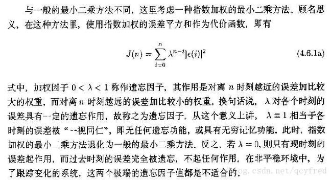
alg = rls(forgetfactor) constructs an adaptive algorithm object based on the recursive least squares (RLS) algorithm. The forgetting factor is forgetfactor, a real number between 0 and 1. The inverse correlation matrix is initialized to a scalar value.
alg = rls(forgetfactor,invcorr0) sets the initialization parameter for the inverse correlation matrix. This scalar value is used to initialize or reset the diagonal elements of the inverse correlation matrix
%% 均衡算法 Demo
% qcy
% matlab自带RLS
% 2017年5月17日15:50:46

clear;
close all;
clc

%%

% The following code illustrates how to use
% equalize with a training sequence.
% The training sequence in this case is just
% the beginning of the transmitted message.

% Set up parameters and signals.
M = 16; % Alphabet size for modulation
msg = randi([0 M-1],2400,1); % Random message
hMod = comm.RectangularQAMModulator(M);
modmsg = step(hMod,msg); % Modulate using M-QAM.
trainlen = 1000; % Length of training sequence
chan = [.986; .845; .237; .123+.31i]; % Channel coefficients
% chan = [1 0.45 0.3+0.2i]; % Channel coefficients

filtmsg = filter(chan,1,modmsg); % Introduce channel distortion.

% Equalize the received signal.
% eq1 = lineareq(40, lms(0.002)); % Create an equalizer object. % 8 taps,lms算法,步长0.01
eq1 = lineareq(40, rls(0.99,0.1)); % Create an equalizer object. % 40 taps,RLS算法,步长0.99,自相关矩阵逆矩阵的对角线初值InvCorrInit
eq1.SigConst = step(hMod,(0:M-1)')'; % Set signal constellation. % 标准星座图
[symbolest,yd] = equalize(eq1,filtmsg,modmsg(1:trainlen)); % Equalize. % 均衡器obj,需要均衡的信号,训练序列

% Plot signals.
h = scatterplot(filtmsg,1,trainlen,'bx'); hold on;
scatterplot(symbolest,1,trainlen,'g.',h);
scatterplot(eq1.SigConst,1,0,'k*',h);
legend('Filtered signal','Equalized signal',...
   'Ideal signal constellation');
hold off;

% Compute error rates with and without equalization.
hDemod = comm.RectangularQAMDemodulator(M);
demodmsg_noeq = step(hDemod,filtmsg); % Demodulate unequalized signal.
demodmsg = step(hDemod,yd); % Demodulate detected signal from equalizer.
hErrorCalc = comm.ErrorRate; % ErrorRate calculator
ser_noEq = step(hErrorCalc, ...
    msg(trainlen+1:end), demodmsg_noeq(trainlen+1:end));
reset(hErrorCalc)
ser_Eq = step(hErrorCalc, msg(trainlen+1:end),demodmsg(trainlen+1:end));
disp('Symbol error rates with and without equalizer:')
disp([ser_Eq(1) ser_noEq(1)])
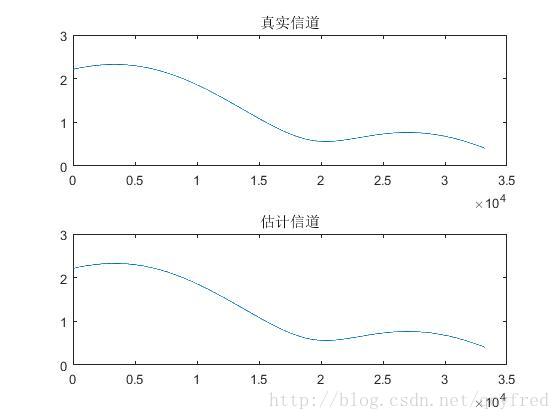
看起来似乎可以完美均衡一样。
close all;
Nfft = 66536;
CHAN = fft(chan,Nfft);
figure;
subplot(211);
plot(abs(CHAN(1:Nfft/2)));
title('真实信道')

subplot(212);
EQ = fft(eq1.Weights,Nfft);
plot(1./abs(EQ(1:Nfft/2)));
title('估计信道')
