Convex Optimization(1)
Introduction
Mathematical Optimization
The basic form:
m i n i m i z e : f 0 ( x ) s u b j e c t t o : f i ( x ) ≤ b i minimize: f_{0}(x)\\ subject\ to: f_{i}(x)\le b_{i} minimize:f0(x)subject to:fi(x)≤bi
. x = ( x 1 , . . . , x n ) : o p t i m i z a t i o n v a r i a b l e s x=(x_{1},...,x_{n}): optimization\ variables x=(x1,...,xn):optimization variables
. f 0 : R n → R : o b j e c t i v e f u n c t i o n f_{0}: R^{n}\to R: objective\ function f0:Rn→R:objective function(可以看作是用来寻找最优解的成本)
. f i : R n → R , i = 1 , . . . , m : c o n s t r a i n t f u n c t i o n f_{i}: R^{n}\to R, i=1,...,m: constraint\ function fi:Rn→R,i=1,...,m:constraint function
optimal solution x ∗ x^{*} x∗ has smallest value of f 0 f_{0} f0 among all vectors that satisfy the constraints.
Application:
. portfolio optimization(投资组合优化)
. device sizing in electronic circuits
. data fitting(数据拟合)
General optimization problem:
. very difficult to solve
. methods involve some compromise, e . g . e.g. e.g., very long computation time, or not always finding the solution.
Exception: certain problem classes can be solved efficiently and reliably
. least-squares problem
. Linear programming
. Convex Optimization
Least-square
The basic form:
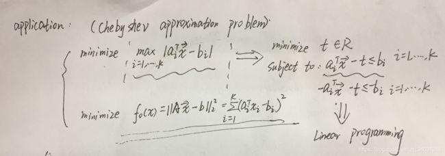
m i n i m i z e : ∥ A x − b ∥ 2 2 = ∑ i = 1 k ( a i T x − b i ) 2 , A ∈ R k × n minimize:\Vert Ax-b\Vert^{2}_{2}=\sum_{i=1}^{k}(a_{i}^{T}x-b_{i})^{2},\ A\in R^{k\times n} minimize:∥Ax−b∥22=i=1∑k(aiTx−bi)2, A∈Rk×n
Solving least-squares problems:
. analytical solution: x ∗ = ( A T A ) − 1 A T b x^{*}=(A^{T}A)^{-1}A^{T}b x∗=(ATA)−1ATb
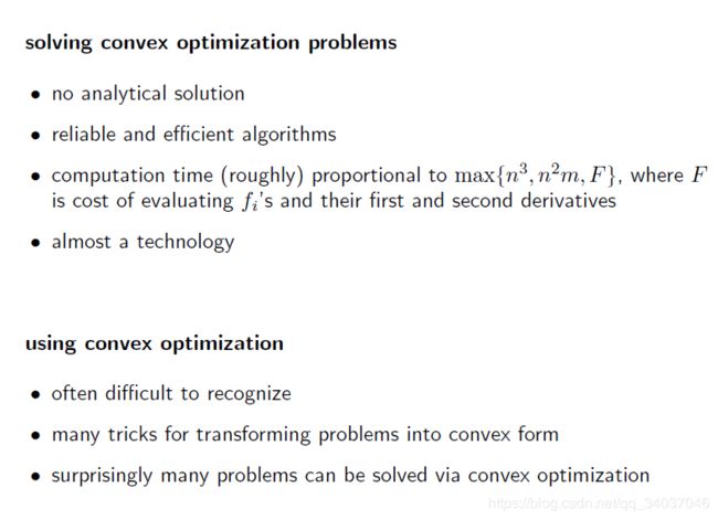
. reliable and efficient algorithms and softwares
. computation time proportional to n 2 k n^{2}k n2k(n is the size of X and K is the number of rows; In other words, K is the number of examples and n is the number of features)
. a mature technology
Using least-squares:
. least-squares problems are very easy to recognize
. a few standard techniques increase flexibility( e . g . , i n c l u d i n g w e i g h t s , a d d i n g r e g u l a r i z a t i o n t e r m s e.g., including weights, adding regularization terms e.g.,includingweights,addingregularizationterms)
Linear Programming
The basic form:
m i n i m i z e : c T x s u b j e c t t o : a i T x ≤ b i , i = 1 , 2 , . . . , m minimize:\ c^{T}x\\ subject\ to:\ a_{i}^{T}x\le b_{i},\ i=1,2,...,m minimize: cTxsubject to: aiTx≤bi, i=1,2,...,m
Solving linear program:
. no analytical formula for solution
. reliable and efficient algorithm and software
. computation time proportional to n 2 m n^{2}m n2m if m ≥ n m\ge n m≥n
. a mature technology
Using linear programming
. not as easy to recognize as least-squares problems
. a few standard tricks used to convert problems into linear programs ( e . g . e.g. e.g., problems involving l 1 − l_{1-} l1− or l ∞ − l_{\infty-} l∞−norms, piecewise-linear functions)
Convex Optimization
The basic form:
m i n i m i z e : f 0 ( x ) s u b j e c t t o : f i ( x ) ≤ b i , i = 1 , 2 , . . . , m minimize: f_{0}(x)\\ subject\ to: f_{i}(x)\le b_{i},\ i=1,2,...,m minimize:f0(x)subject to:fi(x)≤bi, i=1,2,...,m
. objective and constraint functions are convex:
f i ( α x + β y ) ≤ α f i ( x ) + β f i ( y ) , α + β = 1 0 ≤ α ≤ 1 a n d 0 ≤ β ≤ 1 f_{i}(\alpha x+\beta y)\le \alpha f_{i}(x)+\beta f_{i}(y),\ \alpha+\beta=1\\ 0\le \alpha \le1 \ and\ 0\le\beta \le1 fi(αx+βy)≤αfi(x)+βfi(y), α+β=10≤α≤1 and 0≤β≤1
(The least-squares and linear programming is special classes of convex problem. linear problem is like a bowl-shaped thing.If you slice it, you will get ellipsoids(椭圆) and it kind of goes down like that.)

Example


注:1、当最小二乘法使用了包含权重系数的时候,我的理解是:先利用基础的最小二乘法,求得所有的 P j P_{j} Pj,然后将所有的P_{j}中接近或者超过 P m a x P_{max} Pmax的 w j w_{j} wj设置的很高,然后再求的这一次的 P j P_{j} Pj。同理,按照这样的iteration,求得合适的 P j P_{j} Pj,最后使得所有的 P j P_{j} Pj在 P m a x / 2 P_{max}/2 Pmax/2附近“fluctuation”。
2、利用线性规划的求解方法,与上面所提到的切比雪夫估计所使用的方法一致,即式子中包含了 l ∞ 范 数 l_{\infty}范数 l∞范数。


