python+opencv显示图片的直方图、高斯滤波、直方图均衡化的结果
当我们把python和opencv配置好以后我们就可以利用python对图片进行一系列的处理了,看到很多同学都会在pcv上遇到问题,又要去GitHub上面下载pcv,很庆幸自己当时下了anaconda,避免了很多库缺失的问题。
一、python+opencv显示图片的直方图
源代码
from PIL import Image
from pylab import *

# 添加中文字体支持
from matplotlib.font_manager import FontProperties
font = FontProperties(fname=r"c:\windows\fonts\SimSun.ttc", size=14)
im = array(Image.open('hjl.jpg').convert('L'))  # 打开图像,并转成灰度图像

figure()
subplot(121)
gray()
contour(im, origin='image')
axis('equal')
axis('off')
title(u'图像轮廓', fontproperties=font)

subplot(122)
hist(im.flatten(), 128)
title(u'图像直方图', fontproperties=font)
plt.xlim([0,260])
plt.ylim([0,11000])

show()
显示结果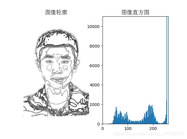
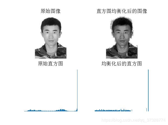
二、python+opencv显示图片的直方图均衡化
源代码
from PIL import Image
from pylab import *
from PCV.tools import imtools

# 添加中文字体支持
from matplotlib.font_manager import FontProperties
font = FontProperties(fname=r"c:\windows\fonts\SimSun.ttc", size=14)

im = array(Image.open('hjl.jpg').convert('L'))  # 打开图像,并转成灰度图像
#im = array(Image.open('hjl.jpg').convert('L'))
im2, cdf = imtools.histeq(im)

figure()
subplot(2, 2, 1)
axis('off')
gray()
title(u'原始图像', fontproperties=font)
imshow(im)

subplot(2, 2, 2)
axis('off')
title(u'直方图均衡化后的图像', fontproperties=font)
imshow(im2)

subplot(2, 2, 3)
axis('off')
title(u'原始直方图', fontproperties=font)
#hist(im.flatten(), 128, cumulative=True, normed=True)
hist(im.flatten(), 128, normed=True)

subplot(2, 2, 4)
axis('off')
title(u'均衡化后的直方图', fontproperties=font)
#hist(im2.flatten(), 128, cumulative=True, normed=True)
hist(im2.flatten(), 128, normed=True)

show()
显示结果
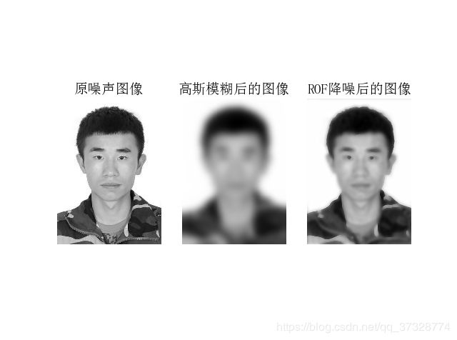
三、python+opencv显示图片的高斯滤波
from numpy import *
from numpy import random
from scipy.ndimage import filters
from scipy.misc import imsave
from PCV.tools import rof

""" This is the de-noising example using ROF in Section 1.5. """

# 添加中文字体支持
from matplotlib.font_manager import FontProperties
font = FontProperties(fname=r"c:\windows\fonts\SimSun.ttc", size=14)

# create synthetic image with noise
im = zeros((500,500))
im[100:400,100:400] = 128
im[200:300,200:300] = 255
im = im + 30*random.standard_normal((500,500))

U,T = rof.denoise(im,im)
G = filters.gaussian_filter(im,10)


# save the result
#imsave('synth_original.pdf',im)
#imsave('synth_rof.pdf',U)
#imsave('synth_gaussian.pdf',G)


# plot
figure()
gray()

subplot(1,3,1)
imshow(im)
#axis('equal')
axis('off')
title(u'原噪声图像', fontproperties=font)

subplot(1,3,2)
imshow(G)
#axis('equal')
axis('off')
title(u'高斯模糊后的图像', fontproperties=font)

subplot(1,3,3)
imshow(U)
#axis('equal')
axis('off')
title(u'ROF降噪后的图像', fontproperties=font)

show()
显示结果