吴恩达机器学习代码及相关知识点总结--ex5(偏差与方差)
1.偏差和方差的定义
偏差:描述的是预测值的期望与真实值之间的差距。偏差越大,越偏离真实数据。
方差:描述的是预测值的变化范围,离散程度,也就是离其期望值的距离,方差越大,数据的分布越分散。
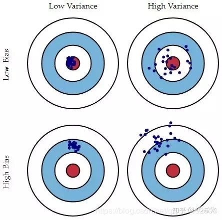

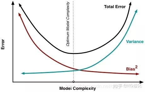
我们训练出来的模型和真实模型之间通常存在着不一致性,而这不一致性就表现为偏差和方差,选择正确的模型复杂的,能够尽可能减少偏差和方差。
复杂度高的模型通常对训练集有很好的拟合能力,但对测试数据就不一定了,极有可能出现过拟合现象,产生较大的偏差。
而复杂度低的模型又不能很好的拟合训练数据,从而产生较大的方差。
模型的复杂度和方差和偏差的关系大致如图所示:
2.如何解决偏差和方差的问题
偏差(欠拟合):
1.寻找更好的特征,使模型更具有代表性
2.用更多的特征即增加输入向量的维度,从而增加模型的复杂度
方差(过拟合):
1.增大数据集
2.减少数据特征,减少输入向量的维度,从而降低模型的复杂度
3.正则化方法:L1,L2正则化,dropout等
4.交叉验证法
3.练习
3.1正则化线性回归
3.1.1数据可视化

import numpy as np
import scipy.io as sio
import scipy.optimize as opt
import pandas as pd
import matplotlib.pyplot as plt
import seaborn as sns
def load_data(path):
    data=sio.loadmat(path)
    return map(np.ravel, [data['X'], data['y'], data['Xval'], data['yval'], data['Xtest'], data['ytest']])
X, y, Xval, yval, Xtest, ytest = load_data("code/ex5-bias vs variance/ex5data1.mat")
df=pd.DataFrame({"water_level":X,"flow":y})
sns.lmplot("water_level","flow",data=df,fit_reg=False,size=7)
plt.show()

3.1.2 正则化线性回归的代价函数
X, Xval, Xtest = [np.insert(x.reshape(x.shape[0], 1), 0, np.ones(x.shape[0]), axis=1) for x in (X, Xval, Xtest)]
#把X, Xval, Xtest中(n,)变为(n,1)再插入x0=1
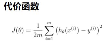
def cost(theta,X,y):
    m=X.shape[0]
    inner=X@theta-y#(12,2)@(2,1)
    cost=(inner@inner.T)/(2*m)
    return cost
def regularized_cost(theta,X,y,l=1):
    m=X.shape[0]
    reg_term=(l/(2*m))*np.sum(np.power(theta[1:],2))
    return cost(theta,X,y)+reg_term
3.1.3正则化梯度下降

def gradient(theta,X,y):
    m=X.shape[0]
    inner=X.T@(X@theta-y)#(n,m)@(m,1)
    return inner/m
def regularized_gradient(theta,X,yy,l=1):
    m=X.shape[0]
    reg_term=theta.copy()
    reg_term[0]=0
    reg_term=(l/m)*reg_term
    return gradient(theta,X,y)+reg_term
regularized_gradient(theta,X,y)
array([-15.30301567, 598.25074417])
3.1.3拟合数据
def linear_regression(X,y,l=1):
     """linear regression
    args:
        X: feature matrix, (m, n+1) # with incercept x0=1
        y: target vector, (m, )
        l: lambda constant for regularization

    return: trained parameters
    """
     theta=np.ones(X.shape[1])
     res=opt.minimize(fun=regularized_cost,x0=theta,args=(X,y,l),method="TNC",jac=regularized_gradient,options={'disp': True})
     return res
res=linear_regression(X, y, l=0)
final_theta=res.x
b = final_theta[0] # intercept
m = final_theta[1] # slope

plt.scatter(X[:,1], y, label="Training data")
plt.plot(X[:, 1], X[:, 1]*m + b, label="Prediction")
plt.legend(loc=2)
plt.show()

可以看到拟合效果并不好,我们再通过学习曲线来观察训练模型。
3.2.1学习曲线
1.为了画出学习曲线我们需要不同尺度的训练集和交叉验证集 Specifically, for
a training set size of i, you should use the first i examples (i.e., X(1:i,:)
and y(1:i)).
2. 训练集误差不包括正则化
3. 交叉验证集的误差需要通过整个交叉验证集来计算
4. 记住使用相同的训练集子集来计算训练代价
training_cost, cv_cost = [], []
m=X.shape[0]
for i in range(1,m+1):
    res=linear_regression(X[:i,:],y[:i],l=0)
    tc=regularized_cost(res.x,X[:i,:],y[:i],l=0)
    cv=regularized_cost(res.x,Xval,yval,l=0)
    training_cost.append(tc)
    cv_cost.append(cv)
plt.plot(np.arange(1, m+1), training_cost, label='training cost')
plt.plot(np.arange(1, m+1), cv_cost, label='cv cost')
plt.legend(loc=1)
plt.show()

可以看出欠拟合,因为我们的模型太简单了,因此我们需要再加入一些特征
3.3.3多项式回归
首先要来创建多项式的特征:

我们需要完成一个函数,使得x从低维映射到高维,即从(m,1)到(m,p),让第一列是原始的x,第二列是x^2,
第三列是 x^3.
准备多项式回归数据:
1.扩展特征到需要的阶数
2.使用 归一化 来合并 x^n
3.don’t forget intercept term
#拓展特征
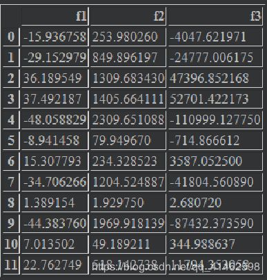
def poly_features(x,power,as_ndarray=False):
data={"f{}".format(i):np.power(x,i) for i in range(1,power+1)}
df=pd.DataFrame(data)
return df.as_matrix() if as_ndarray else df
#加载数据
X, y, Xval, yval, Xtest, ytest = load_data("code/ex5-bias vs variance/ex5data1.mat")
poly_features(X,3)
#归一化
def normalize_feature(df):
    return df.apply(lambda column:(column-column.mean())/column.std())
def prepare_poly_data(*args, power):
    """
    args: keep feeding in X, Xval, or Xtest
        will return in the same order
    """
    def prepare(x):
        # expand feature
        df = poly_features(x, power=power)

        # normalization
        ndarr = normalize_feature(df).as_matrix()

        # add intercept term
        return np.insert(ndarr, 0, np.ones(ndarr.shape[0]), axis=1)

    return [prepare(x) for x in args]
X_poly, Xval_poly, Xtest_poly= prepare_poly_data(X, Xval, Xtest, power=8)
X_poly[:3, :]
array([[ 1.00000000e+00, -3.62140776e-01, -7.55086688e-01,
1.82225876e-01, -7.06189908e-01, 3.06617917e-01,
-5.90877673e-01, 3.44515797e-01, -5.08481165e-01],
[ 1.00000000e+00, -8.03204845e-01, 1.25825266e-03,
-2.47936991e-01, -3.27023420e-01, 9.33963187e-02,
-4.35817606e-01, 2.55416116e-01, -4.48912493e-01],
[ 1.00000000e+00, 1.37746700e+00, 5.84826715e-01,
1.24976856e+00, 2.45311974e-01, 9.78359696e-01,
-1.21556976e-02, 7.56568484e-01, -1.70352114e-01]])
def plot_learning_curve(X,y,Xval,yval,l=0):
    m=X.shape[0]
    training_cost=[]
    cv_cost=[]
    for i in range(1,m+1):
        res=linear_regression(X[:i,:],y[:i],l=1)
        tc=cost(res.x,X[:i,:],y[:i])
        cv=cost(res.x,Xval,yval)
        training_cost.append(tc)
        cv_cost.append(cv)
    plt.plot(np.arange(1,m+1),training_cost,label="training cost")
    plt.plot(np.arange(1,m+1),cv_cost,label="cv cost")
    plt.legend(loc=1)
plot_learning_curve(X_poly, y, Xval_poly, yval, l=0)
plt.show()

可以看到没有正则化的时候,training cost为0,此时出现过拟合
将正则化系数改为1时:

训练代价不再是0了,减轻了过拟合现象
plot_learning_curve(X_poly, y, Xval_poly, yval, l=100)
plt.show()

欠拟合了
寻找最适合的正则化参数
l_candidate = [0, 0.001, 0.003, 0.01, 0.03, 0.1, 0.3, 1, 3, 10]
training_cost, cv_cost = [], []
for l in l_candidate:
    res = linear_regression(X_poly, y, l)

    tc = cost(res.x, X_poly, y)
    cv = cost(res.x, Xval_poly, yval)

    training_cost.append(tc)
    cv_cost.append(cv)
plt.plot(l_candidate, training_cost, label='training')
plt.plot(l_candidate, cv_cost, label='cross validation')
plt.legend(loc=2)

plt.xlabel('lambda')

plt.ylabel('cost')
plt.show()

# use test data to compute the cost
for l in l_candidate:
    theta = linear_regression(X_poly, y, l).x
    print('test cost(l={}) = {}'.format(l, cost(theta, Xtest_poly, ytest)))
test cost(l=0) = 10.122298845834932
test cost(l=0.001) = 10.989357236615056
test cost(l=0.003) = 11.26731092609127
test cost(l=0.01) = 10.881623900868235
test cost(l=0.03) = 10.02232745596236
test cost(l=0.1) = 8.632062332318977
test cost(l=0.3) = 7.336513212074589
test cost(l=1) = 7.466265914249742
test cost(l=3) = 11.643931713037912
test cost(l=10) = 27.7150802906621
可以看出在l=0.3时最小