数字图像处理(灰度变换与空间滤波)
灰度变换与空间滤波
- 术语:空间域
- 空间域处理的表示:
- 术语:空间滤波器
- 灰度变换(点处理技术)
- 灰度变换函数
- 线性函数
- 对数函数
- 伽马变换
- 对比度拉伸变换函数
- 阈值处理函数
- 分段线性变换
- IPT提供的API
- imadjust
- stretchlim
- 灰度变换的一些实用M函数
- 处理可变数目的输入或输出
- intrans函数的实现
- 亮度标度的M函数:gscale
- 直方图处理
- 直方图均衡
- 直方图匹配
- 空间滤波基础
- 线性空间滤波器
- 一般形式:
- 示意图:
- 空间相关与卷积
- 空间相关
- 相关操作的公式:
- 与离散单位冲击作用:
- 空间卷积
- 相关操作的公式:
- 与离散单位冲击作用:
- 代码实现
- IPT提供的API
- 平滑空间滤波器/均值滤波器/低通滤波器
- 锐化空间滤波器
- 作用:
- 基础:
- 定义:
- 图像锐化的拉普拉斯算子
- 滤波器模板
- 拉普拉斯图像锐化
- 例:
- 非锐化掩蔽与高提升滤波
- 梯度法
- 非线性空间滤波器
- 统计排序滤波器
- IPT的标准空间滤波器
- fspecial
- ordfilt2
- medfilt2
- 参考文献:
术语:空间域
空间域指图像平面本身,这是相对于变换域而言的,变换域的图像处理首先把空间域变换到变换域,在变换域中处理图像,再通过反变换,把处理结果返回到空间域。
空间域的图像处理直接对图像中的像素进行操作,主要分为灰度变换和空间滤波。
空间滤波也称领域处理或空间卷积。
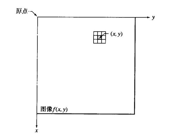
空间域处理的表示:
g ( x , y ) = T [ f ( x , y ) ] g(x,y)=T[f(x,y)] g(x,y)=T[f(x,y)]
-
f(x,y)是输入图像,g(x,y) 是输出图像,T 是在点 (x,y) 的邻域上定义的关于 f 的一种算子。
-
T 可作用于单幅图像,也可作用于图像集合,如为了降低噪声而对图像序列执行逐像素求和操作。
-
领域通常取为以 (x,y) 为中心的矩形领域,大小为 ( 2 a + 1 ) × ( 2 b + 1 ) (2a+1)\times(2b+1) (2a+1)×(2b+1) 。
-
空间滤波的过程:领域中心从图像原点开始,从左到右,从上到下移动,输出图像在每一个空间坐标 (x,y)
处的像素值就是 T 作用在 f 的以 (x,y) 为中心的领域上所得的值。note:当邻域中心充分靠近图像边界时,部分领域会位于图像外部,此时需要做一些技术处理,主要有以下两种方法:
- 忽略外侧邻点
- 用0或者其他指定灰度值填充图像边缘
术语:空间滤波器
领域与预定义的操作 T 一起称为空间滤波器,也称空间掩模,核,模板或窗口。
灰度变换(点处理技术)
当领域取为最小领域 1 × 1 1\times 1 1×1 时,g 仅取决于 (x,y) 处的 f 值与算子 T .此时空间域处理可以简单得表示成:
s = T ( r ) s=T(r) s=T(r)
- r,s 分别表示 f,g 在任意点 (x,y) 的灰度
灰度变换函数
线性函数
-
恒等变换
不改变图像,仅出于理论完整性考虑 -
反转变换
-
表达式:
s = L − 1 − r s=L-1-r s=L−1−r -
此处假设灰度级范围是[0 , L-1]
-
作用:可以得到等效的照片底片,适用于增强嵌入在暗区域中白色或灰色细节,特别是黑色占主导地位时。
-
代码实现:
function g = imreverse(f) %IMREVERSE computes the negative of an image f % Convert the image to uint8_type f_uint8 = im2uint8(f); g = 255 - f_uint8; -
效果展示:
input:>> f = imread('Fig0304(a)(breast_digital_Xray).tif'); >> g = imreverse(f); >> figure >> subplot(1,2,1);imshow(f),title('原图'); >> subplot(1,2,2);imshow(g),title('图像反转');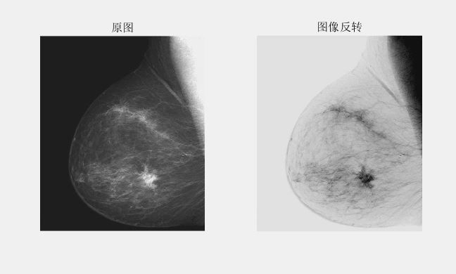
-
对数函数
- 通用形式:
s = c l o g ( 1 + r ) s = clog(1+r) s=clog(1+r) - c是常数,假设 r ≥ 0 r\ge 0 r≥0
- 图像:
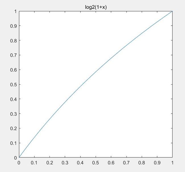
- 从对数曲线的形状可以看出,该变换将较窄范围的暗色输入值映射为较宽范围的输出值,将较宽范围的亮色输入值映射为较窄范围的输出值。
- 代码实现:
function g = imlog(f) %IMLOG takes the logarithm transform of an image f f1 = mat2gray(im2double(f)); g = log2(1+f1); - 效果展示:
 >> f = imread('Fig0316(4)(bottom_left).tif');
 >> g = imlog(f);
 >> figure
 >> subplot(1,2,1);imshow(f),title('原图');
 >> subplot(1,2,2);imshow(g),title('log');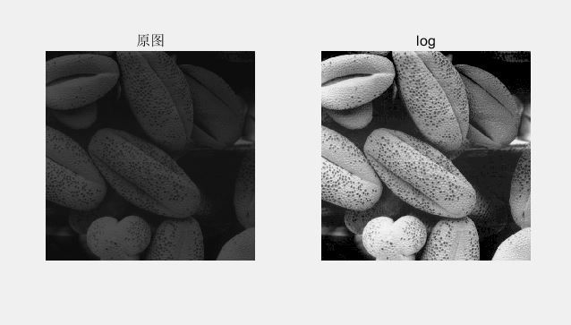
- 作用:
- 放大低灰度值区域的细节
- 压缩动态范围
例:当因为数值范围过大,导致图像显示效果不佳时,可以利用对数运算将大范围压缩到小范围这一性质,做对数变换后,再显示图像。
以下原图是范围在0到1.5\times 10^6 的傅里叶频谱,频谱中的低值损失严重。做对数变换后,效果好很多。f = imread('Fig0305(a)(DFT_no_log).tif'); g = im2uint8(mat2gray(log(1+double(f)))); figure subplot(1,2,1);imshow(f),title('原图'); subplot(1,2,2);imshow(g),title('log');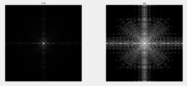
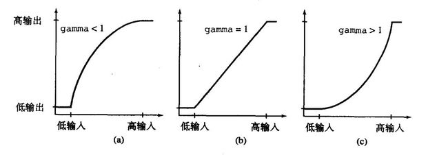
伽马变换
-
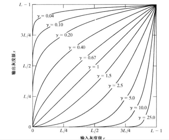
基本形式:
s = c r γ s = cr^{\gamma} s=crγ- c, γ \gamma γ 是正常数
- γ > 1 \gamma > 1 γ>1 时,该变换将较窄范围的暗色输入值映射为较宽范围的输出值,将较宽范围的亮色输入值映射为较窄范围的输出值。
γ < 1 \gamma<1 γ<1 时,效果相反 - 不同 γ \gamma γ 值下,曲线的形状:
-
代码实现:
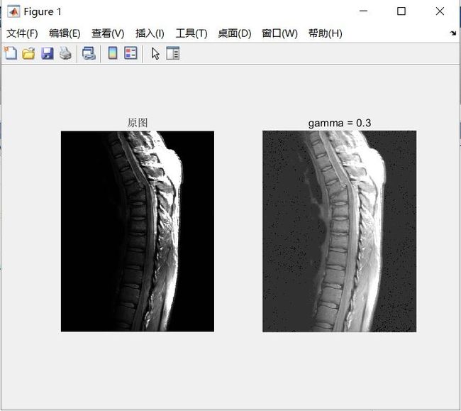
M文件:function g = imgamma(f, gamma) %IMGAMMA takes a gamma transform of an image f % First, we normalizes the pixel value of the image f to [0,1] f1 = double(f); f2 = mat2gray(f1); g = f2.^gamma;例:
input:>> f = imread('Fig0308(a)(fractured_spine).tif'); >> g = imgamma(f,0.3); >> figure >> subplot(1,2,1);imshow(f),title('原图'); >> subplot(1,2,2);imshow(g),title('gamma = 0.3');output:
-
应用:
-
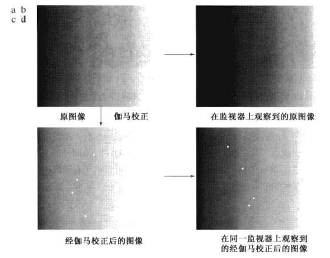
伽马校正:用于图像获取,打印和显示的各种设备自身根据伽马变换产生响应。显示系统的这一特性会使显示的图像和原图像相比偏暗或偏亮。这时根据设备的伽马值做相应的伽马变换,称为伽马校正,使得设备能正确显示原图。
例:下图是监视器上显示图像的伽马校正过程。因为CRT有一个灰度-电压响应,相当于显示图像时自动做了一个 γ \gamma γ 值在1.8到2.5的伽马变换,使得监视器显示的图像偏暗。在显示图像前,先对原图做一个伽马值等于 1 γ \frac{1}{\gamma} γ1 的伽马变换作为校正,这样监视器就能正确显示原图像了。
-
对比度增强:
例:有时图像偏暗,可以使用 γ < 1 \gamma <1 γ<1 的伽马变换。为了使得显示效果最佳,通常要尝试不同的 γ \gamma γ 值。
γ \gamma γ 越接近1,图像越接近原图; γ \gamma γ 越接近0,原图暗处的细节被增强,但对比度降低,图像容易被"冲淡"。f = imread('Fig0308(a)(fractured_spine).tif'); gamma = [0.6 0.4 0.3]; figure subplot(1,4,1);imshow(f),title('原图'); for i = 1:3 g = imgamma(f,gamma(i)); subplot(1,4,i+1);imshow(g),title(gamma(i)); end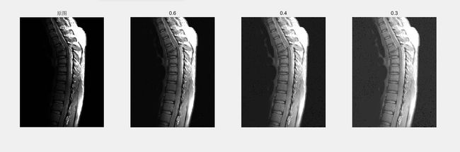
γ = 0.3 \gamma = 0.3 γ=0.3 时,黑色背景已出现很多灰点, γ = 0.4 \gamma=0.4 γ=0.4 效果最好例:有时图像偏亮,可以使用 γ > 1 \gamma >1 γ>1 的伽马变换。为了使得显示效果最佳,通常要尝试不同的 γ \gamma γ 值。
γ \gamma γ 越接近1,图像越接近原图,但原图偏亮,图像有"冲淡"的外观; γ \gamma γ 越接近无穷,原图越暗,太暗会丢失细节。f = imread('Fig0309(a)(washed_out_aerial_image).tif'); gamma = [3 4 5]; figure subplot(1,4,1);imshow(f),title('原图'); for i = 1:3 g = imgamma(f,gamma(i)); subplot(1,4,i+1);imshow(g),title(gamma(i)); end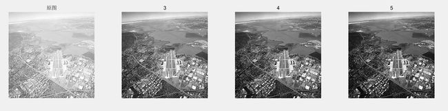
γ = 5 \gamma = 5 γ=5 时,图像已经偏暗,暗处细节已经丢失, γ = 4 \gamma=4 γ=4 效果最好
-
对比度拉伸变换函数
-
基本形式:
s = T ( r ) = 1 1 + ( m / r ) E s=T(r)=\frac{1}{1+(m/r)^E} s=T(r)=1+(m/r)E1- 参数 E,m 控制函数的形状
-
图像:
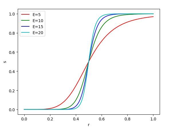
可以看出:这个变换将小于 m 的输入灰度级压缩到靠近0的窄区域,将大于 m 的输入灰度级压缩到靠近1的窄区域,使得输出具有高对比度。E越小,压缩效果越小;E越大,压缩能力越大,图像越向二值图像靠近。 -
代码实现
function g = imContrasStretch(f, m, E) %IMCONTRASSTRETCH takes the ContrasStretch tansform of an image f % m is the x-value of the inflection point % E determines the steepness of the curve f1 = mat2gray(im2double(f)); g = 1./(1+(m./(f1+eps)).^E); -
效果展示:
 >> f = imread('rose_512.tif');
 >> g = imContrasStretch(f,0.5,20);
 >> figure
 >> subplot(1,2,1);imshow(f),title('原图');
 >> subplot(1,2,2);imshow(g),title('对比度拉伸');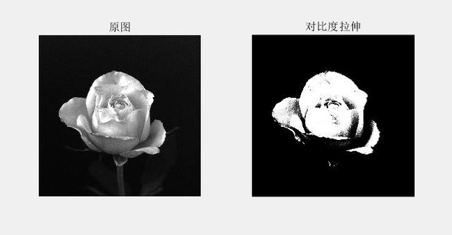
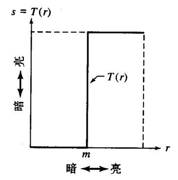
阈值处理函数
- 基本形式:
s = { 0 r < m 1 r ≥ m s=\left\{ \begin{array}{rcl} 0 & & {r<m}\\ 1 & & {r\ge m}\\ \end{array} \right. s={01r<mr≥m- 将输入图像变为二值图像,像素值小于 m 变换为0,大于或等于 m 变换为1
- 图像:
- 代码实现:
function g = myIm2bw(f,T) %MYIM2BW turns an image f into a logical image % T is the threshold that belongs to [0,1] f1 = mat2gray(im2double(f)); g = (f1 >= T); - 效果展示及与MATLAB内置函数im2bw对比
 >> f = imread('rose_512.tif');
 >> g1 = myIm2bw(f,0.5);
 >> g2 = im2bw(f,0.5);
 >> figure
 >> subplot(1,3,1);imshow(f),title('原图');
 >> subplot(1,3,2);imshow(g1),title('myIm2bw');
 >> subplot(1,3,3);imshow(g2),title('Im2bw');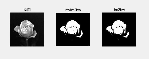
- 应用:图像分割
分段线性变换
- 优点:可以任意复杂,满足各种需求。
- 缺点:要求用户寻找合适的函数
- 应用:
-
对比度拉伸:扩展图像灰度级动态范围
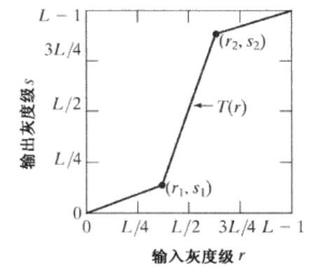
- 例:构造以下灰度变换(像素值归一化为[0,1])
s = { ( s 1 / r 1 ) ⋅ r r < r 1 s 2 − s 1 r 2 − r 1 ( r − r 1 ) + s 1 r 1 ≤ r ≤ r 2 1 − s 2 1 − r 2 ( r − r 2 ) + s 2 r > r 2 s=\left\{ \begin{array}{rcl} (s_1/r_1)\cdot r& & {r<r_1}\\ \frac{s_2-s_1}{r_2-r_1}(r-r_1)+s_1 & & {r_1\le r\le r_2}\\ \frac{1-s_2}{1-r_2}(r-r_2)+s_2& & {r>r_2} \end{array} \right. s=⎩⎨⎧(s1/r1)⋅rr2−r1s2−s1(r−r1)+s11−r21−s2(r−r2)+s2r<r1r1≤r≤r2r>r2
- 例:构造以下灰度变换(像素值归一化为[0,1])
-
图像:
-
代码实现
function g = imcontras(f,r1,s1,r2,s2) %IMCONTRAS take the piecewise linear transform of an image f % r1 -
效果展示
  >> f = imread('Fig0320(2)(2nd_from_top).tif');
  >> g = imcontras(f,0.3,0.125,0.6,0.875);
  >> figure
  >> subplot(1,2,1);imshow(f),title('原图');
  >> subplot(1,2,2);imshow(g),title('分段线性变换后');
-
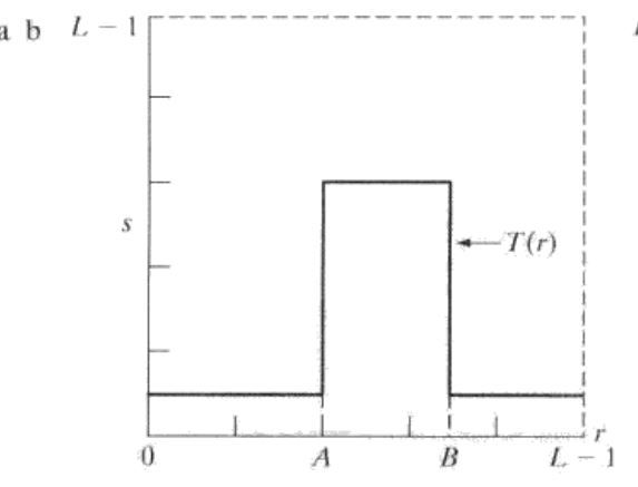
灰度级分层
作用:突出特定灰度范围
基本方法1:将感兴趣的灰度值变为1或者接近1,其他值变为0或者接近0- 图像:
- 代码实现:
function g = imlayered(f,r1,s1,r2,s2) %IMCONTRAS take the piecewise linear transform of an image f % r1 - 效果展示
 f = imread('Fig0235(c)(kidney_original).tif');
 g = imlayered(f,0.7,0,0.9,1);
 figure
 subplot(1,2,1);imshow(f),title('原图');
 subplot(1,2,2);imshow(g),title('灰度分层后');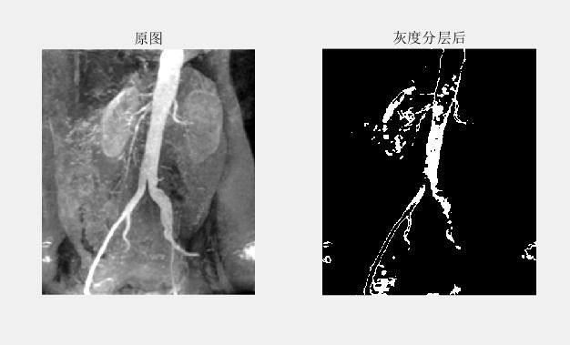
基本方法2:将感兴趣的灰度值变为1或者接近1,其他值不变 - 图像:

- 代码实现
function g = imlayered2(f,r1,r2,s) %IMCONTRAS take the piecewise linear transform of an image f % r1r2 g(i,j) = ff(i,j); else g(i,j) = s; end end end - 效果展示
 f = imread('Fig0235(c)(kidney_original).tif');
 g = imlayered2(f,0.6,0.9,1);
 figure
 subplot(1,2,1);imshow(f),title('原图');
 subplot(1,2,2);imshow(g),title('灰度分层后');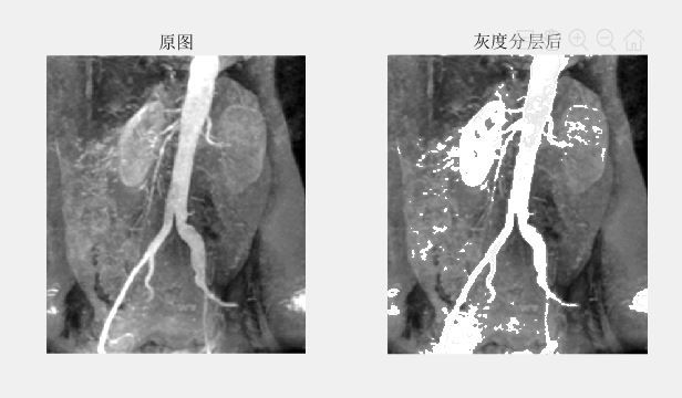
- 图像:
-
比特平面分层
- 作用:突出特定比特
术语:比特平面:对于一个8比特的图像,共8层比特平面,第 i ( i = 2 , 3 , . . . , 8 ) i(i=2,3,...,8) i(i=2,3,...,8) 层比特平面指像素值在 [ 2 i − 1 , 2 i − 1 ] [2^{i-1},2^{i}-1] [2i−1,2i−1], 第一层是 { 0 , 1 } \{0,1\} {0,1}
- 总结:低比特平面像素值范围小,包含的图像信息少,它们主要贡献更精细的细节
高比特平面像素值范围大,包含了图像的主要信息 - 代码实现
function imBitLayer(f) %IMBITLAYER receive an image f and return its bitplanes ff = im2uint8(f); [M,N] = size(f); for k = 2:8 g(:,:,k) = zeros(M,N); for i = 1:M for j = 1:N if ff(i,j)>=2^(k-1) && ff(i,j)<=2^k-1 g(i,j,k)=1; end end end end for i = 1:M for j = 1:N if ff(i,j)==0 || ff(i,j)==1 g(i,j,1)=1; end end end figure subplot(3,3,1);imshow(f),title('原图'); for i = 2:9 subplot(3,3,i);imshow(g(:,:,i-1)),title(i-1); end - 效果展示
 >> f = imread('Fig0314(a)(100-dollars).tif');
 >> imBitLayer(f)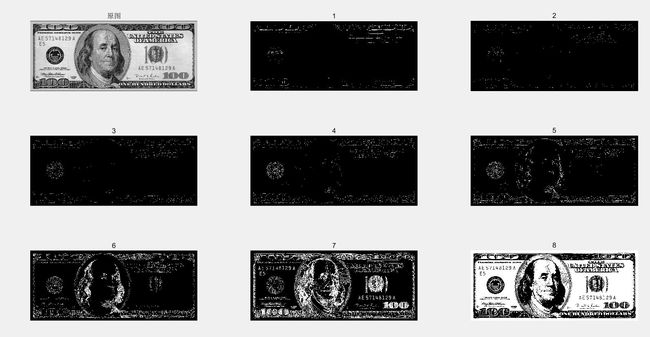
-
IPT提供的API
imadjust
-
语法:
g = i m a d j u s t ( f , [ l o w _ i n , h i g h _ i n ] , [ l o w _ o u t , h i g h _ o u t ] , g a m m a ) g=imadjust(f,[low\_in,high\_in],[low\_out,high\_out],gamma) g=imadjust(f,[low_in,high_in],[low_out,high_out],gamma) -
输入图像应属于uint8,uint16或double类。输出图像与输入图像同类型。
-
[low_in,high_in] , [low_out , high_out] 都是[0,1]的子区间,若设置为[],则表示[0,1]
它们与gamma共同决定了一个分段幂律变换,公式如下:
不妨记:[ low_in , high_in] = [a,b] , [low_out , high_out]=[c,d] , gamma= γ \gamma γ
g = { c f < a ( d − c ) ( f − a b − a ) γ + c a ≤ f ≤ b d f > b g=\left\{ \begin{array}{rcl} c & & {f<a}\\ (d-c)(\frac{f-a}{b-a})^{\gamma}+c & & {a\le f\le b}\\ d & & {f>b} \end{array} \right. g=⎩⎨⎧c(d−c)(b−af−a)γ+cdf<aa≤f≤bf>b -
参数gamma指明了曲线形状。gamma<1, 映射加权至较高输出值 ;gamma>1,映射加权至较低输出值。gamma默认为1
-
imadjust先将 f 归一化,再代入上述公式计算g ,最后根据 f 的类型将g的值还原为相应的范围,过程中遇到需要取整时就取整。
-
特别地,high_out可以小于low_out,此时输出亮度将反转
-
imadjust可以实现图像反转,伽马变换和某些分段线性变换
-
例:以下图片是一幅数字乳房X射线图像,显示出一处病灶,原图偏亮的病灶嵌在一大片黑色区域中,不利于分析病情,使用imadjust做图像增强处理。
   >> f = imread('Fig0304(a)(breast_digital_Xray).tif');
   >> g1 = imadjust(f,[0,1],[1,0]);
   >> g2 = imadjust(f,[0.5 0.75],[0 1]);
   >> g3 = imadjust(f,[],[],2);
   >> figure
   >> subplot(1,4,1);imshow(f),title('原始图像');
   >> subplot(1,4,2);imshow(g1),title('g1');
   >> subplot(1,4,3);imshow(g2),title('g2');
   >> subplot(1,4,4);imshow(g3),title('g3');
输出:
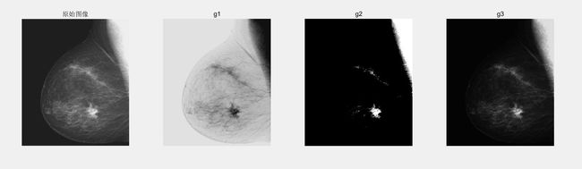
- g1是原图的图像反转
- g2是将原图位于[0.5 , 0.75]之间的亮度扩展到[0 , 1],用于强调图像中感兴趣的亮度区域。
- g3是原图的伽马变换,压缩了低端,扩展了高端
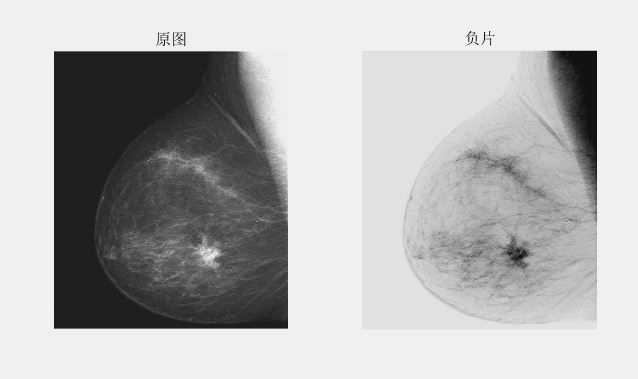
note: 函数imcomplement也可以得到图像反转。
   >> f = imread('Fig0304(a)(breast_digital_Xray).tif');
   >> g = imcomplement(f);
   >> figure
   >> subplot(1,2,1);imshow(f),title('原图');
   >> subplot(1,2,2);imshow(g),title('负片');
输出:
stretchlim
用于自动设置imadjust的[ low_in , high_in]
-
语法:
L o w _ H i g h = s t r e t c h l i m ( f , t o l ) Low\_High = stretchlim(f , tol) Low_High=stretchlim(f,tol)- 如果tol是二维向量[low_frac , high_frac],指定了图像低和高像素值饱和度的百分比。
- 如果tol是标量,那么[low_frac , high_frac] = [tol, 1-tol]
- tol默认为[0.01,0.99]
- tol = 0,low_high = [min(f( : )) , max(f( : ))]
-
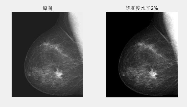
例:
 >> f = imread('Fig0304(a)(breast_digital_Xray).tif');
 >> g = imadjust(f,stretchlim(f),[]);
 >> figure
 >> subplot(1,2,1);imshow(f),title('原图');
 >> subplot(1,2,2);imshow(g),title('饱和度水平2%');
输出:
灰度变换的一些实用M函数
处理可变数目的输入或输出
- nargin: 返回输入到M函数的输入变量数
- nargout: 返回M函数的输出变量数
- nargchk:
- 语法:
m s g = n a r g c h k ( l o w , h i g h , n u m b e r ) msg=nargchk(low,high,number) msg=nargchk(low,high,number)- 检查传递的参数数量是否正确
- number
- 语法:
- varargin/varargout: 用于可变数量的参数,以单元数组的形式存储
intrans函数的实现
-
代码:
function g = intrans(f, varargin) %INTRANS Performs intensity (gray-level) transformations. % G = INTRANS(F, 'neg') computes the negative of input image F. % % G = INTRANS(F, 'log', C, CLASS) computes C*log(1 + F) and % multiplies the result by (positive) constant C. If the last two % parameters are omitted, C defaults to 1. Because the log is used % frequently to display Fourier spectra, parameter CLASS offers the % option to specify the class of the output as 'uint8' or % 'uint16'. If parameter CLASS is omitted, the output is of the % same class as the input. % % G = INTRANS(F, 'gamma', GAM) performs a gamma transformation on % the input image using parameter GAM (a required input). % % G = INTRANS(F, 'stretch', M, E) computes a contrast-stretching % transformation using the expression 1./(1 + (M./(F + % eps)).^E). Parameter M must be in the range [0, 1]. The default % value for M is mean2(im2double(F)), and the default value for E % is 4. % % For the 'neg', 'gamma', and 'stretch' transformations, double % input images whose maximum value is greater than 1 are scaled % first using MAT2GRAY. Other images are converted to double first % using IM2DOUBLE. For the 'log' transformation, double images are % transformed without being scaled; other images are converted to % double first using IM2DOUBLE. % % The output is of the same class as the input, except if a % different class is specified for the 'log' option. % Verify the correct number of inputs. error(nargchk(2, 4, nargin)) % Store the class of the input for use later. classin = class(f); % If the input is of class double, and it is outside the range % [0, 1], and the specified transformation is not 'log', convert the % input to the range [0, 1]. if strcmp(class(f), 'double') & max(f(:)) > 1 & ... ~strcmp(varargin{1}, 'log') f = mat2gray(f); else % Convert to double, regardless of class(f). f = im2double(f); end % Determine the type of transformation specified. method = varargin{1}; % Perform the intensity transformation specified. switch method case 'neg' g = imcomplement(f); case 'log' if length(varargin) == 1 c = 1; elseif length(varargin) == 2 c = varargin{2}; elseif length(varargin) == 3 c = varargin{2}; classin = varargin{3}; else error('Incorrect number of inputs for the log option.') end g = c*(log(1 + double(f))); case 'gamma' if length(varargin) < 2 error('Not enough inputs for the gamma option.') end gam = varargin{2}; g = imadjust(f, [ ], [ ], gam); case 'stretch' if length(varargin) == 1 % Use defaults. m = mean2(f); E = 4.0; elseif length(varargin) == 3 m = varargin{2}; E = varargin{3}; else error('Incorrect number of inputs for the stretch option.') end g = 1./(1 + (m./(f + eps)).^E); otherwise error('Unknown enhancement method.') end % Convert to the class of the input image. g = changeclass(classin, g); -
例:
 f = imread('Fig0306(a)(bone-scan-GE).tif');
 g = intrans(f,'stretch',mean2(im2double(f)),0.9);
 figure
 subplot(1,2,1);imshow(f),title('原图');
 subplot(1,2,2);imshow(g),title('stretch');
亮度标度的M函数:gscale
-
代码:
function g = gscale(f, varargin) %GSCALE Scales the intensity of the input image. % G = GSCALE(F, 'full8') scales the intensities of F to the full % 8-bit intensity range [0, 255]. This is the default if there is % only one input argument. % % G = GSCALE(F, 'full16') scales the intensities of F to the full % 16-bit intensity range [0, 65535]. % % G = GSCALE(F, 'minmax', LOW, HIGH) scales the intensities of F to % the range [LOW, HIGH]. These values must be provided, and they % must be in the range [0, 1], independently of the class of the % input. GSCALE performs any necessary scaling. If the input is of % class double, and its values are not in the range [0, 1], then % GSCALE scales it to this range before processing. % % The class of the output is the same as the class of the input. if length(varargin) == 0 % If only one argument it must be f. method = 'full8'; else method = varargin{1}; end if strcmp(class(f), 'double') & (max(f(:)) > 1 | min(f(:)) < 0) f = mat2gray(f); end % Perform the specified scaling. switch method case 'full8' g = im2uint8(mat2gray(double(f))); case 'full16' g = im2uint16(mat2gray(double(f))); case 'minmax' low = varargin{2}; high = varargin{3}; if low > 1 | low < 0 | high > 1 | high < 0 error('Parameters low and high must be in the range [0, 1].') end if strcmp(class(f), 'double') low_in = min(f(:)); high_in = max(f(:)); elseif strcmp(class(f), 'uint8') low_in = double(min(f(:)))./255; high_in = double(max(f(:)))./255; elseif strcmp(class(f), 'uint16') low_in = double(min(f(:)))./65535; high_in = double(max(f(:)))./65535; end % imadjust automatically matches the class of the input. g = imadjust(f, [low_in high_in], [low high]); otherwise error('Unknown method.') end -
语法:
g = g s c a l e ( f , m e t h o d , l o w , h i g h ) g=gscale(f,method,low,high) g=gscale(f,method,low,high)- method取值:
- ‘full8’(默认),省略low,high, 像素值标度到[0,255]
- ‘full16’, 省略low,high, 像素值标度到[0,65535]
- ‘minmax’, 必须有low,high ([0,1]之间)
- method取值:
直方图处理
-
数字图像的直方图:
h ( r k ) = n k h(r_k)=n_k h(rk)=nk- 离散函数
- 灰度级范围 [0,G] ,共 L 个级别。
- r_k 表示第 k 级灰度值,n_k 表示图像中灰度为 r_k 的像素个数。
-
归一化直方图:
p ( r k ) = n k / M N p(r_k)=n_k/MN p(rk)=nk/MN- 它是各级灰度在图像中出现的频率统计
- 若将灰度级 r_k 看成一个随机变量,则它是 r_k 的概率分布列的一个估计
-
应用:
- 图像增强
- 图像压缩
- 图像分割
-
代码实现:
M文件:function hist(f) %HIST gives the histogram of an image f % First convert the image to uint8 f_uint8 = im2uint8(f); [M, N] = size(f); MN = M * N; r = 0:255; n = zeros(1,256); for i = 1:256 n(i) = sum(sum(f_uint8 == (i-1)))/MN; end plot(r, n) xlim([0, 255]) -
IPT提供的API
imhist:>> f = imread('Fig0306(a)(bone-scan-GE).tif'); >> imhist(f)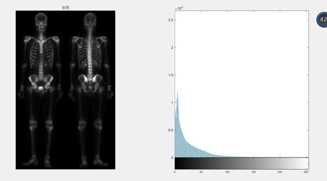
-
例:
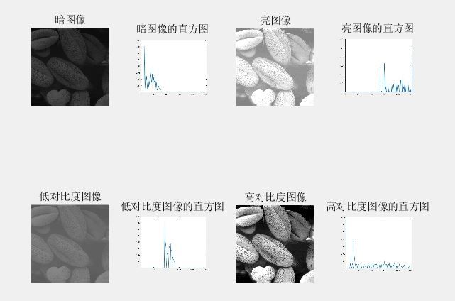
从上图中可以看出:
-
暗图像的直方图集中在低灰度端
-
亮图像的直方图集中在高灰度端
-
低对比度图像的直方图集中在中间
-
高对比度图像的直方图分布均匀,覆盖范围广
总结:
若一幅图像的像素分布接近于整个灰度级上的均匀分布,则图像会有高对比度,灰色调变化较大,最终效果是一幅灰度细节丰富,动态范围较大的图像。
直方图均衡
目标:找一个灰度变换,使得变换后的图像的直方图接近整个灰度范围上的均匀分布,以此得到高对比度,动态范围广的图像。
step1: 目标灰度变换需满足的必要条件:(假设灰度级归一化为 [0,1] )
s = T ( r ) s=T(r) s=T(r)
- T ( r ) T(r) T(r) 在区间 [0,1] 上单调增
这是为了防止出现灰度反转,造成人为缺陷。 - T ( r ) T(r) T(r) 的值域也是 [0,1]
这是保证输入输出的灰度范围相同
step2: 假设输入 r ,输出 s 均为 [0,1] 上随机变量, p r ( r ) , p s ( s ) p_r(r),p_s(s) pr(r),ps(s) 分别是它们的概率密度函数,则令:
s = ∫ 0 r p r ( w ) d w s=\int_0^r p_r(w)dw s=∫0rpr(w)dw
由概率密度函数非负和归一化条件知step1中条件满足
由概率论可知:
p s ( s ) = p r ( r ) ∣ d r d s ∣ d s d r = p r ( r ) p s ( s ) = p r ( r ) 1 p r ( r ) = 1 \begin{aligned} & p_s(s)=p_r(r)|\frac{dr}{ds}|\\ & \frac{ds}{dr}=p_r(r)\\ & p_s(s)=p_r(r)\frac{1}{p_r(r)}=1 \end{aligned} ps(s)=pr(r)∣dsdr∣drds=pr(r)ps(s)=pr(r)pr(r)1=1
说明在上述灰度变换下,s服从 [0,1] 上的均匀分布
step3: 离散化
数字图像的灰度值总是离散的,用求和代替积分,求出离散形式的灰度变换函数
s k = T ( r k ) = ∑ j = 1 k p r ( r j ) = ∑ j = 1 k n j n , k = 1 , 2 , . . . L s_k=T(r_k)=\sum\limits_{j=1}^kp_r(r_j)=\sum\limits_{j=1}^k\frac{n_j}{n}\ ,k=1,2,...L sk=T(rk)=j=1∑kpr(rj)=j=1∑knnj ,k=1,2,...L
由于连续时, s 是 [0,1] 到 [0,1] 的单调增函数,离散化,再还原为原灰度范围(必要时四舍五入)后, s k s_k sk 仍然满足条件
例:假设一幅大小为 64 × 64 64\times 64 64×64 像素的3比特图像,灰度级为 [0,7] 中的整数,具体信息如下:
| 灰度级 | 归一化灰度级 | rk | nk | pr(rk) | sk | sk(四舍五入)转化到原灰度级范围 |
|---|---|---|---|---|---|---|
| 0 | 0 | r1 | 790 | 0.19 | 0.19 | 1.33取1 |
| 1 | 0.125 | r2 | 1023 | 0.25 | 0.44 | 3.08取3 |
| 2 | 0.25 | r3 | 850 | 0.21 | 0.65 | 4.55取5 |
| 3 | 0.375 | r4 | 656 | 0.16 | 0.81 | 5.67取6 |
| 4 | 0.5 | r5 | 329 | 0.08 | 0.89 | 6.23取6 |
| 5 | 0.625 | r6 | 245 | 0.06 | 0.95 | 6.65取7 |
| 6 | 0.75 | r7 | 122 | 0.03 | 0.98 | 6.86取7 |
| 7 | 0.875 | r8 | 81 | 0.02 | 1 | 7.00取7 |
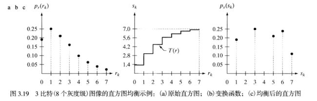
note: 离散化后,直方图只是概率密度的近似,不能证明离散直方图均衡能导出均匀的直方图,但这种变换有展开输入图像直方图的趋势,均衡化后的灰度级更宽了,最终效果是增强了对比度。
IPT提供的API:
histeq
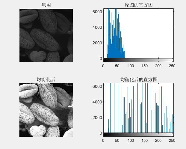
例
 f = imread('Fig0316(4)(bottom_left).tif');
 g = histeq(f,256);
 figure
 subplot(2,2,1);imshow(f),title('原图');
 subplot(2,2,2);imhist(f),title('原图的直方图');
 subplot(2,2,3);imshow(g),title('均衡化后');
 subplot(2,2,4);imhist(g),title('均衡化后的直方图');
直方图匹配
目标:找一个灰度变换,使得变换后的图像的直方图是我们预定的直方图,这个预定是我们根据需求确定的。
step1: 先做直方图均衡,将r变换成s,s服从[0,1]上均匀分布
s = T ( r ) s=T(r) s=T(r)
step2: 假设z是服从我们预定的直方图的随机变量,则对z做直方图均衡,同样得到s
s = G ( z ) s=G(z) s=G(z)
step3: 求逆
要求G满足:
-
G(z) 在区间 [0,1] 上严格单调增
为了保证G的反函数存在 -
G(z) 的值域也是 [0,1]
这是保证输入输出的灰度范围相同求逆得:
z = G − 1 [ T ( r ) ] z = G^{-1}[T(r)] z=G−1[T(r)]
是我们要得变换
step4: 离散化
实践中我们处理的是离散值,最终得到预定直方图的一个近似
先有直方图均衡得到:
s k = T ( r k ) s k = G ( z q ) s_k=T(r_k)\\ s_k=G(z_q) sk=T(rk)sk=G(zq)
根据这两个对应关系可得:
z q = G − 1 [ T ( r k ) ] z_q=G^{-1}[T(r_k)] zq=G−1[T(rk)]
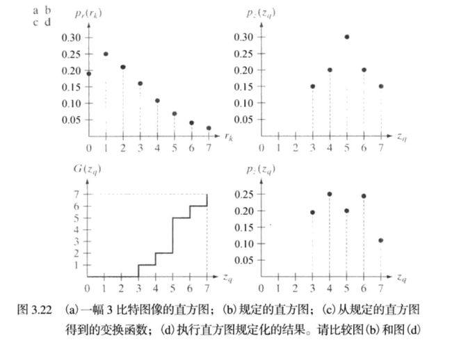
例:假设一幅大小为 64 × 64 64\times 64 64×64 像素的3比特图像,灰度级为 [0,7] 中的整数,具体信息如下:
| 像素值 | 实际的pr | 规定的pz | r到s | z到s | r到z |
|---|---|---|---|---|---|
| 0 | 0.19 | 0.00 | 1 | 0 | 3 |
| 1 | 0.25 | 0.00 | 3 | 0 | 4 |
| 2 | 0.21 | 0.00 | 5 | 0 | 5 |
| 3 | 0.16 | 0.15 | 6 | 1 | 6 |
| 4 | 0.08 | 0.20 | 6 | 2 | 6 |
| 5 | 0.06 | 0.30 | 7 | 5 | 7 |
| 6 | 0.03 | 0.20 | 7 | 6 | 7 |
| 7 | 0.02 | 0.15 | 7 | 7 | 7 |
实际中不需要G可逆,因为我们处理的是离散值,由r去找对应的s, 由s去找那些z与s对应,如果有多个,取与r最近的那个,如果没有相应的z, 就重新找与r对应的s, 找最接近的。
-
IPT提供的API:
histeq:
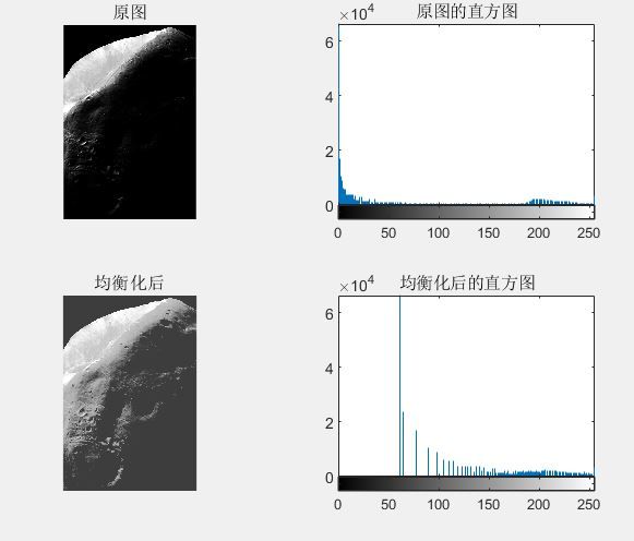
 f = imread('Fig0323(a)(mars_moon_phobos).tif');
 ff = histeq(f,256);

 figure
 subplot(2,2,1);imshow(f),title('原图');
 subplot(2,2,2);imhist(f),title('原图的直方图');
 subplot(2,2,3);imshow(ff),title('均衡化后');
 subplot(2,2,4);imhist(ff),title('均衡化后的直方图');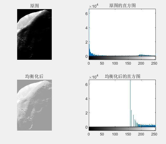
均衡化后效果并不好,因为原图集中在暗色区,使得离散化的灰度变换很快达到最大灰度值,均衡化后,集中到了亮色区
使用直方图匹配改进:
原图的直方图有两个峰值,大的靠近0,小的靠近255,我们用两个峰值的高斯函数拟合这种直方图图像
多峰值高斯函数:
 function p = twomodegauss(m1, sig1, m2, sig2, A1, A2, k)
 %TWOMODEGAUSS Generates a two-mode Gaussian function.
 %   P = TWOMODEGAUSS(M1, SIG1, M2, SIG2, A1, A2, K) generates a
 %   two-mode, Gaussian-like function in the interval [0,1].  P is a
 %   256-element vector normalized so that SUM(P) equals 1.  The mean
 %   and standard deviation of the modes are (M1, SIG1) and (M2,
 %   SIG2), respectively. A1 and A2 are the amplitude values of the
 %   two modes.  Since the output is normalized, only the relative
 %   values of A1 and A2 are important.  K is an offset value that
 %   raises the "floor" of the function.  A good set of values to try
 %   is M1=0.15, S1=0.05, M2=0.75, S2=0.05, A1=1, A2=0.07, and
 %   K=0.002.

 c1 = A1 * (1 / ((2 * pi) ^ 0.5) * sig1);
 k1 = 2 * (sig1 ^ 2);
 c2 = A2 * (1 / ((2 * pi) ^ 0.5) * sig2);
 k2 = 2 * (sig2 ^ 2);
 z  = linspace(0, 1, 256);

 p = k + c1 * exp(-((z - m1) .^ 2) ./ k1) + ...
     c2 * exp(-((z - m2) .^ 2) ./ k2);
 p = p ./ sum(p(:));
 p = twomodegauss(0.15, 0.05, 0.75, 0.05, 1, 0.07, 0.002);
 f = imread('Fig0323(a)(mars_moon_phobos).tif');
 g = histeq(f,p);
 figure
 subplot(2,2,1);imshow(f),title('原图');
 subplot(2,2,2);imhist(f),title('原图的直方图');
 subplot(2,2,3);imshow(g),title('均衡化后');
 subplot(2,2,4);imhist(g),title('均衡化后的直方图');
空间滤波基础
线性空间滤波器
在图像像素上执行线性操作的滤波器称为线性空间滤波器
一般形式:
假设领域大小取成 m × n = ( 2 a + 1 ) × ( 2 b + 1 ) m\times n=(2a+1)\times(2b+1) m×n=(2a+1)×(2b+1) ,a,b 是正整数。
g ( x , y ) = ∑ u = − a u = a ∑ v = − b v = b w ( u , v ) f ( x + u , y + v ) g(x,y)=\sum\limits_{u=-a}^{u=a}\sum\limits_{v=-b}^{v=b}w(u,v)f(x+u,y+v) g(x,y)=u=−a∑u=av=−b∑v=bw(u,v)f(x+u,y+v)
示意图:

空间相关与卷积
术语:离散单位冲激:包含一个1,其余全是0的函数。
空间相关
相关操作的公式:
w ( x , y ) ☆ f ( x , y ) = ∑ u = − a u = a ∑ v = − b v = b w ( u , v ) f ( x + u , y + v ) w(x,y)☆f(x,y)=\sum\limits_{u=-a}^{u=a}\sum\limits_{v=-b}^{v=b}w(u,v)f(x+u,y+v) w(x,y)☆f(x,y)=u=−a∑u=av=−b∑v=bw(u,v)f(x+u,y+v)
- 对所有位移量 x,y 求值
- 在靠近边界处,需要填充 f
与离散单位冲击作用:
- 离散单位冲击与滤波器如下:
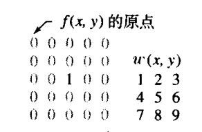
- 进行相关操作:

- 裁剪后最终结果:
在1的位置生成一个翻转180度的滤波器
空间卷积
相关操作的公式:
w ( x , y ) ∗ f ( x , y ) = ∑ u = − a u = a ∑ v = − b v = b w ( u , v ) f ( x − u , y − v ) w(x,y)*f(x,y)=\sum\limits_{u=-a}^{u=a}\sum\limits_{v=-b}^{v=b}w(u,v)f(x-u,y-v) w(x,y)∗f(x,y)=u=−a∑u=av=−b∑v=bw(u,v)f(x−u,y−v)
- 对所有位移量 x,y 求值
- 在靠近边界处,需要填充 f
- 相当于w先翻转180°,再做相关
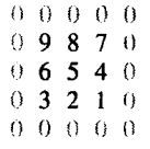
与离散单位冲击作用:
- 离散单位冲击与滤波器如下:
- 进行相关操作:
- 裁剪后最终结果:
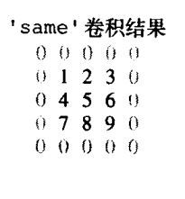
在1的位置生成一个滤波器
代码实现
  function g = myImfilter(f, w, filter_mode, bd_type, size_option)
  %MYIMFILTER implements the linear space filtering operation of an image f
  % f is the input image
  % g is the output image
  % w is a linear space filter, which is given by users. The size of w must
  % be odd
  % filter_mode has two options, 'corr'and 'conv',which indicate
  % the relevant and the convolution operation respectly
  % bd_type has four options
  % p , a value, means fill f with p(The default is 0)
  % 'rep' means fill f with the boundary value
  % 'sym' means image size expanding by mirroring their boundaries
  % 'cir' means fill f periodicly
  % size_option has two options
  % 'full' outputs extended g
  % 'same' outputs g with the same size of f

  % get the size oof w
  [m,n] = size(w);
  if mod(m*n,2)==0
      error('The size of w must be odd')
  end

  % choose flipping w or not based on filter_mode
  if strcmp(filter_mode,'corr')
      ww = w;
  else
      ww = rot90(w,2);
  end

  %fill f according to the option of bd_type
  a = (m-1)/2;
  b = (n-1)/2;
  [M,N] = size(f);
  ff = zeros(M + 2*a, N + 2*b);
  ff((a+1):(a+M),(b+1):(b+N)) = f(:,:);
  if strcmp(bd_type,'rep')
      for i = 1:a
          ff(i,(b+1):(b+N)) = f(1,:);
      end
      for i = (a+M+1):(2*a + M)
          ff(i,(b+1):(b+N)) = f(M,:);
      end
      for j = 1:b
          ff(:,j) = ff(:,b+1);
      end
      for j = (b+N+1):(2*b+N)
          ff(:,j) = ff(:,b+M);
      end
  elseif strcmp(bd_type,'sym')
      for i = 1:a
          ff(i,(b+1):(b+N)) = f(a+1-i,:);
      end
      for i = 1:a
          ff(a+M+i,(b+1):(b+N)) = f(M-i+1,:);
      end
      for j = 1:b
          ff(:,j) = ff(:,2*b+1-i);
      end
      for j = 1:b
          ff(:,b+N+j) = ff(:,b+N+1-j);
      end
  elseif strcmp(bd_type,'cir')
      for i = 1:a
          ff(i,(b+1):(b+N)) = f(M-a+i,:);
      end
      for i = 1:a
          ff(a+M+i,(b+1):(b+N)) = f(i,:);
      end
      for j = 1:b
          ff(:,j) = ff(:,N+j);
      end
      for j = 1:b
          ff(:,b+N+j) = ff(:,b+j);
      end
  else
      p = bd_type;
      for i = 1:a
          ff(i,(b+1):(b+N)) = ones(1,N).*p;
      end
      for i = 1:a
          ff(a+M+i,(b+1):(b+N)) = ones(1,N).*p;
      end
      for j = 1:b
          ff(:,j) = ones(M+2*a,1).*p;
      end
      for j = 1:b
          ff(:,b+N+j) = ones(M+2*a,1).*p;
      end
  end

  gg = zeros(M+2*a,N+2*b);
  for i = (a+1):(a+M)
      for j = (b+1):(b+N)
          gg(i,j) = sum(sum(ww.* ff((i-a):(i+a),(j-b):(j+b))));
      end
  end

  if strcmp(size_option, 'full')
      g = gg;
  else
      g = zeros(M,N);
      g = gg((a+1):(a+M),(b+1):(b+N));
  end
IPT提供的API
imfilter
-
语法:
g = i m f i l t e r ( f , w , f i l t e r _ m o d e , b o u n d a r y _ o p t i o n s , s i z e _ o p t i o n s ) g = imfilter(f,w,filter\_mode,boundary\_options,size\_options) g=imfilter(f,w,filter_mode,boundary_options,size_options)- f 是输入图像
- w是滤波器
- filter_mode 是选择操作模式,‘ corr ’ 代表相关,‘ conv ’ 代表卷积
- boundary_options 是选择填充边界的方式,数值p表示用p填充,‘replicate’ 表示用边界值扩展,‘symmetric’ 表示镜像反射边界进行扩展,‘circular’ 表示将数组当成二维周期函数扩展
- size_options 是选择输出模式,‘full’ 输出扩展的数组,‘same’ 输出与输入同样大小的裁剪数组
-
不同模式处理结果对比:
 f = imread('Fig0216(a).tif');
 w = ones(31)./(31^2);
 g1 = imfilter(f,w,'corr','same');
 g2 = imfilter(f,w,'corr','replicate','same');
 g3 = imfilter(f,w,'corr','symmetric','same');
 g4 = imfilter(f,w,'corr','circular','same');
 figure
 subplot(3,2,[1,2]);imshow(f),title('原图');
 subplot(3,2,3);imshow(g1,[]),title('0填充');
 subplot(3,2,4);imshow(g2,[]),title('replicate');
 subplot(3,2,5);imshow(g3,[]),title('symmetric');
 subplot(3,2,6);imshow(g4,[]),title('circular');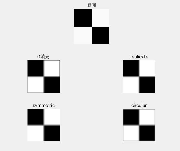
此处w对称,所以相关和卷积结果一样,分析上图可以看出,w是一个平滑滤波器note:imfilter会将输出图像转化为输入图像的类型,比如,输入图像是‘uint8’,w没有归一化,计算可能超出255,最终会被imfliter截断,导致输出异常,如下图。因此,使用时注意将w归一化
 f = imread('Fig0216(a).tif');
 w = ones(31);
 g1 = imfilter(f,w,'corr','same');
 figure
 subplot(1,2,1);imshow(f),title('原图');
 subplot(1,2,2);imshow(g1,[]),title('0填充');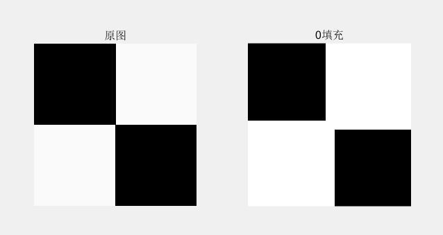
平滑空间滤波器/均值滤波器/低通滤波器
- 作用:模糊处理与降噪
- w系数求和为1:滤波时,相当于对 (x,y) 邻域里的所有像素值做加权平均。
特别的,w系数相同,相当于做简单平均,此时也称为盒状滤波器 - 例:
 f = imread('Fig0333(a)(test_pattern_blurring_orig).tif');
 m = [3 5 9 15 35];
 figure
 subplot(2,3,1);imshow(f),title('原图');
 for i = 1:5
     w = ones(m(i))./(m(i)^2);
     g = imfilter(f,w,'corr','same');
     subplot(2,3,i+1);
     imshow(g),title(m(i));
 end
当图像有锯齿的时候,可以选择平滑滤波器,从上图可以看出,邻域取得越大,模糊效果越明显,需要根据图像情况,选择合适的滤波器大小。
锐化空间滤波器
作用:
突出图像中过渡部分
基础:
图像的一阶微分与二阶微分
一阶微分要求:
- 在恒定灰度值区域,微分为零
- 在灰度台阶或斜坡处非零
- 沿着斜坡的微分值非零
二阶微分要求:
- 在一阶微分值恒定区域,二阶微分为零
- 在灰度台阶或斜坡起点处非零
- 沿着斜坡二阶微分值为零
这些要求是从连续情形下,微分的性质类比而来,在离散情形下,此处的一阶微分实指差分
定义:
f 在 (x,y) 处的一阶微分:
∂ f ∂ x = f ( x + 1 , y ) − f ( x , y ) ∂ f ∂ y = f ( x , y + 1 ) − f ( x , y ) \frac{\partial f}{\partial x}=f(x+1,y)-f(x,y)\quad \frac{\partial f}{\partial y}=f(x,y+1)-f(x,y) ∂x∂f=f(x+1,y)−f(x,y)∂y∂f=f(x,y+1)−f(x,y)
f 在 (x,y) 处的二阶微分:
∂ 2 f ∂ 2 x = f ( x + 1 , y ) + f ( x − 1 , y ) − 2 f ( x , y ) ∂ 2 f ∂ 2 y = f ( x , y + 1 ) + f ( x , y − 1 ) − 2 f ( x , y ) \frac{\partial^2 f}{\partial^2 x}=f(x+1,y)+f(x-1,y)-2f(x,y)\quad\frac{\partial^2 f}{\partial^2 y}=f(x,y+1)+f(x,y-1)-2f(x,y) ∂2x∂2f=f(x+1,y)+f(x−1,y)−2f(x,y)∂2y∂2f=f(x,y+1)+f(x,y−1)−2f(x,y)
图像锐化的拉普拉斯算子
∇ 2 f ( x , y ) = ∂ 2 f ∂ 2 x + ∂ 2 f ∂ 2 y = f ( x + 1 , y ) + f ( x − 1 , y ) + f ( x , y + 1 ) + f ( x , y − 1 ) − 4 f ( x , y ) \nabla^2f(x,y) =\frac{\partial^2 f}{\partial^2 x}+\frac{\partial^2 f}{\partial^2 y}=f(x+1,y)+f(x-1,y)+f(x,y+1)+f(x,y-1)-4f(x,y) ∇2f(x,y)=∂2x∂2f+∂2y∂2f=f(x+1,y)+f(x−1,y)+f(x,y+1)+f(x,y−1)−4f(x,y)
术语:各向同性滤波器是指旋转不变的滤波器,w具有旋转不变性。
滤波器模板
由上述拉普拉斯算子可以得到如下滤波器模板
w = 0 1 0 1 − 4 1 0 1 0 w= \begin{matrix} 0 & 1 & 0 \\ 1 & -4 & 1 \\ 0 & 1 & 0 \end{matrix} w=0101−41010
这是一个以90°为增量的各向同性模板
例:找一个以45°为增量的各项同性模板
在拉普拉斯算子的基础上加入对角线方向,形成算子:
T = f ( x + 1 , y + 1 ) + f ( x + 1 , y ) + f ( x − 1 , y ) + f ( x − 1 , y − 1 ) + f ( x , y + 1 ) + f ( x , y − 1 ) + f ( x + 1 , y − 1 ) + f ( x − 1 , y + 1 ) − 8 f ( x , y ) \begin{aligned} T & =f(x+1,y+1)+f(x+1,y)+f(x-1,y)+f(x-1,y-1)\\ & +f(x,y+1)+f(x,y-1)+f(x+1,y-1)+f(x-1,y+1)\\ & -8f(x,y) \end{aligned} T=f(x+1,y+1)+f(x+1,y)+f(x−1,y)+f(x−1,y−1)+f(x,y+1)+f(x,y−1)+f(x+1,y−1)+f(x−1,y+1)−8f(x,y)
模板为
w = 1 1 1 1 − 8 1 1 1 1 w= \begin{matrix} 1 & 1 & 1 \\ 1 & -8 & 1 \\ 1 & 1 & 1 \end{matrix} w=1111−81111
拉普拉斯图像锐化
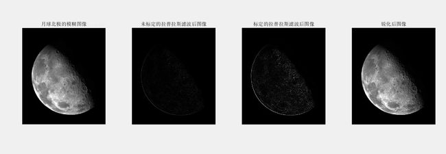
原图像减去拉普拉斯变换后的图像可以复原背景特性并保持拉普拉斯锐化处理效果
g ( x , y ) = f ( x , y ) + c ∇ 2 f ( x , y ) g(x,y)=f(x,y)+c\nabla^2f(x,y) g(x,y)=f(x,y)+c∇2f(x,y)
若w中心系数为负,则取c=-1;反之,取c=1
例:
   f = imread('Fig0338(a)(blurry_moon).tif');
   w = [0 1 0;1 -4 1;0 1 0];
   delta_f = imfilter(f,w,'corr','same');
   delta_f_scale = gscale(delta_f,'full8');
   g = f-delta_f;
   figure
   subplot(1,4,1);imshow(f),title('月球北极的模糊图像');
   subplot(1,4,2);imshow(delta_f),title('未标定的拉普拉斯滤波后图像');
   subplot(1,4,3);imshow(delta_f_scale),title('标定的拉普拉斯滤波后图像');
   subplot(1,4,4);imshow(g),title('锐化后图像');
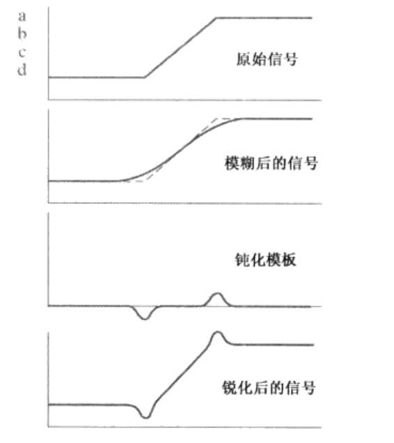
非锐化掩蔽与高提升滤波
- 模糊原图像
- 从原图像中减去模糊图像(称为模板)
- 原图像加上权重模板
公式:
g ( x , y ) = f ( x , y ) + k ( f ( x , y ) − f ∗ ( x , y ) ) g(x,y)=f(x,y)+k(f(x,y)-f^*(x,y)) g(x,y)=f(x,y)+k(f(x,y)−f∗(x,y)) - f ∗ ( x , y ) f^*(x,y) f∗(x,y) 是模糊后的图像
- k ≥ 0 k\ge 0 k≥0
- k=1时称为非锐化掩蔽;k>1时称为高提升滤波;k<1时不强调模板的贡献
图像说明:
术语:高斯平滑滤波器是指w由二维高斯函数生成的滤波器
例:
 f = imread('Fig0340(a)(dipxe_text).tif');
 % 生成高斯平滑滤波器,sigma=3
 w = zeros(5,5);
 for i = 1:5
     for j = 1:5
         w(i,j) = exp(-((i-3)^2+(j-3)^2)/18);
     end
 end
 ww = w./25;
 gauss_f = imfilter(f,ww,'corr','same')
 g_mask = f-gauss_f;
 g1 = f+g_mask;
 g45 = f+4.5.*g_mask;

 figure
 subplot(1,5,1);imshow(f),title('原图');
 subplot(1,5,2);imshow(gauss_f),title('高斯模糊后的结果');
 subplot(1,5,3);imshow(g_mask),title('模板');
 subplot(1,5,4);imshow(g1),title('非锐化掩蔽');
 subplot(1,5,5);imshow(g45),title('k=4.5的高提升滤波');

梯度法
-
图像梯度:
∇ f = [ ∂ f ∂ x , ∂ f ∂ y ] T \nabla f=[\frac{\partial f}{\partial x},\frac{\partial f}{\partial y}]^T ∇f=[∂x∂f,∂y∂f]T -
梯度幅值:
M ( x , y ) = ( f x 2 + f y 2 ) M(x,y)=\sqrt{(f_x^2+f_y^2)} M(x,y)=(fx2+fy2)
图像 M(x,y) 称为梯度图像 -
例:
sobel算子:( 3 × 3 3\times 3 3×3模板)- 梯度近似:
g x = ( z 7 + 2 z 8 + z 9 ) − ( z 1 + 2 z 2 + z 3 ) g y = ( z 3 + 2 z 6 + z 9 ) − ( z 1 + 2 z 4 + z 7 ) g_x=(z_7+2z_8+z_9)-(z1+2z_2+z_3)\\ g_y=(z_3+2z_6+z_9)-(z1+2z_4+z_7) gx=(z7+2z8+z9)−(z1+2z2+z3)gy=(z3+2z6+z9)−(z1+2z4+z7)- x方向用第3行减第1行近似梯度
- y方向用第3列减第1列近似梯度
- 中间系数用2是为了保证模板系数和为0,从而满足灰度恒定区域,梯度为0
- 模板
w x = [ − 1 − 2 − 1 0 0 0 1 2 1 ] w_x= \begin{bmatrix} -1 & -2 & -1 \\ 0 & 0 & 0 \\ 1 & 2 & 1 \end{bmatrix} wx=⎣⎡−101−202−101⎦⎤
w y = [ − 1 0 1 − 2 0 2 − 1 0 1 ] w_y= \begin{bmatrix} -1 & 0 & 1 \\ -2 & 0 & 2 \\ -1 & 0 & 1 \end{bmatrix} wy=⎣⎡−1−2−1000121⎦⎤
这两个模板称为soble算子
- 梯度近似:
-
梯度图像
M ( x , y ) ≈ ∣ ( z 7 + 2 z 8 + z 9 ) − ( z 1 + 2 z 2 + z 3 ) ∣ + ∣ ( z 3 + 2 z 6 + z 9 ) − ( z 1 + 2 z 4 + z 7 ) ∣ M(x,y) \approx |(z_7+2z_8+z_9)-(z1+2z_2+z_3)|+|(z_3+2z_6+z_9)-(z1+2z_4+z_7)| M(x,y)≈∣(z7+2z8+z9)−(z1+2z2+z3)∣+∣(z3+2z6+z9)−(z1+2z4+z7)∣ -
例:使用梯度进行边缘增强
   f = imread('Fig0342(a)(contact_lens_original).tif');
   % soble算子
   wx = [-1 -2 -1;0 0 0 ;1 2 1]./9;
   wy = [-1 0 1;-2 0 2;-1 0 1]./9;
   fx = imfilter(f,wx,'corr','same');
   fy = imfilter(f,wy,'corr','same');
   M = abs(fx)+abs(fy);

   figure
   subplot(1,2,1);imshow(f),title('原图');
   subplot(1,2,2);imshow(M),title('梯度图像');
原图是一个玻璃镜片,右下角有一个缺口,进行边缘增强后,缺口更明显
非线性空间滤波器
统计排序滤波器
- 中值滤波器:(x,y) 处的输出像素值是它邻域内像素值的中值
- 最大值滤波器: (x,y) 处的输出像素值是它邻域内像素值的最大值
- 最小值滤波器:(x,y) 处的输出像素值是它邻域内像素值的最小值
中值滤波器有很好的去噪能力
术语:椒盐噪声:以黑白点的形式叠加在图像上
IPT的标准空间滤波器
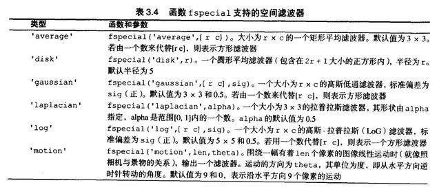
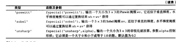
fspecial
生成线性滤波器
- 语法:
w = f s p e c i a l ( ′ t y p e ′ , p a r a m e t e r s ) w = fspecial('type',parameters) w=fspecial(′type′,parameters)
参数取值如下:
- 例
用fspecial生成一个拉普拉斯滤波器,对图像进行锐化w = fspecial('laplacian',0); f = imread('Fig0338(a)(blurry_moon).tif'); ff = im2double(f); g = imfilter(ff,w,'replicate'); g2 = ff-g; figure subplot(1,3,1);imshow(f),title('月球北极的模糊图像'); subplot(1,3,2);imshow(g),title('拉普拉斯滤波后图像'); subplot(1,3,3);imshow(g2),title('图像锐化');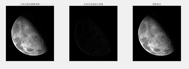
ordfilt2
生成统计排序滤波器
- 语法:
g = o r d f i l t 2 ( f , o r d , d o m a i n ) g = ordfilt2(f,ord,domain) g=ordfilt2(f,ord,domain)- f输入图像
- ord取排序后第几百分位代替邻域中心处的值
- domain 由0,1组成的 m × n m\times n m×n 矩阵,0处的值不参与排序
- 例:
- 最大值滤波器:
g = o r d f i l t 2 ( f , m ∗ n , o n e s ( m , n ) ) g = ordfilt2(f,m*n,ones(m,n)) g=ordfilt2(f,m∗n,ones(m,n)) - 最小值滤波器
g = o r d f i l t 2 ( f , 1 , o n e s ( m , n ) ) g = ordfilt2(f,1,ones(m,n)) g=ordfilt2(f,1,ones(m,n)) - 中值滤波器
g = o r d f i l t 2 ( f , m e d i a n ( 1 : m ∗ n ) , o n e s ( m , n ) ) g = ordfilt2(f,median(1:m*n),ones(m,n)) g=ordfilt2(f,median(1:m∗n),ones(m,n))
- 最大值滤波器:
medfilt2
二维中值滤波函数
- 语法:
g = m e f i l t 2 ( f , [ m , n ] , p a d o p t ) g = mefilt2(f,[m,n],padopt) g=mefilt2(f,[m,n],padopt)- [m,n]邻域大小
- padopt
- ‘zeros’ 零填充(默认)
- ‘symmetric’ 镜像对称填充
- ‘indexed’ 如果是double类,则1填充,否则0填充
- 例:去除椒盐噪声
 f = imread('Fig0335(a)(ckt_board_saltpep_prob_pt05).tif');
 g = medfilt2(f);
 g2 = medfilt2(f,'symmetric');

 figure
 subplot(1,3,1);imshow(f),title('原图');
 subplot(1,3,2);imshow(g),title('0填充');
 subplot(1,3,3);imshow(g2),title('镜像对称填充');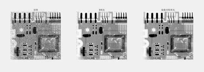
参考文献:
《数字图像处理》第三版
《数字图像处理MATLAB版》