Python金融大数据分析——第7章 输入/输出操作 笔记
- 第7章 输入/输出操作
- 7.1 Python基本I/O
- 7.1.1 将对象写入磁盘
- 7.1.2 读写文本文件
- 7.1.3 SQL数据库
- 7.1.4 读写NumPy数组
- 7.2 Pandas的I/O
- 7.2.1 SQL数据库
- 7.2.2 从SQL到pandas
- 7.2.3 CSV文件数据
- 7.2.4 Excel文件数据
- 7.1 Python基本I/O
- 7.3 PyTables的快速I/O
-
- 7.3.1 使用表
- 7.3.2 使用压缩表
- 7.3.3 使用数组
- 7.3.4 内存外计算
-
第7章 输入/输出操作
7.1 Python基本I/O
7.1.1 将对象写入磁盘
path = 'E:/Projects/python_for_finance/data/'
import numpy as np
from random import gauss

a = [gauss(1.5, 2) for i in range(1000000)]
import pickle

pkl_file = open(path + 'data.pkl', 'wb')
%time pickle.dump(a, pkl_file)
# Wall time: 50 ms
pkl_file
# <_io.BufferedWriter name='E:/Projects/python_for_finance/data/data.pkl'>
pkl_file.close()

pkl_file=open(path+'data.pkl','rb')
%time b=pickle.load(pkl_file)
# Wall time: 83 ms
pkl_file.close()
b[:5]
# [1.9033590575256176,
#  3.511418163957323,
#  -1.8127871618469182,
#  4.3331914411815955,
#  0.17676737228711303]

a[:5]
# [1.9033590575256176,
#  3.511418163957323,
#  -1.8127871618469182,
#  4.3331914411815955,
#  0.17676737228711303]

np.allclose(np.array(a),np.array(b))
# True

np.sum(np.array(a)-np.array(b))
# 0.0

# pickle 存储两个对象
pkl_file=open(path+'data.pkl','wb')
%time pickle.dump(np.array(a),pkl_file)
# Wall time: 63 ms
%time pickle.dump(np.array(a)**2,pkl_file)
# Wall time: 52 ms
pkl_file.close()

pkl_file=open(path+'data.pkl','rb')
# 第一次调用pickle.load返回第一个对象
x=pickle.load(pkl_file)
x
# array([ 1.90335906,  3.51141816, -1.81278716, ...,  2.54216848,
#         1.10891189, -1.41041133])
# 第二次调用pickle.load返回第二个对象
y=pickle.load(pkl_file)
y
# array([  3.6227757 ,  12.33005752,   3.28619729, ...,   6.46262057,
#          1.22968557,   1.98926012])
pkl_file.close()
# pickle按照先进先出(FIFO)原则保存对象

# 推荐使用字典进行一次存取,如下:
pkl_file=open(path+'data.pkl','wb')
pickle.dump({'x': x, 'y': y}, pkl_file)
pkl_file.close()

pkl_file = open(path+'data.pkl','rb')
data = pickle.load(pkl_file)
pkl_file.close()
for key in data.keys():
    print(key,data[key][:4])
# x [ 1.90335906  3.51141816 -1.81278716  4.33319144]
# y [  3.6227757   12.33005752   3.28619729  18.77654807]
7.1.2 读写文本文件
rows = 5000
a = np.random.standard_normal((rows, 5))
a.round(4)
# array([[-0.2789, -0.0167, -1.5313,  0.0687,  1.3295],
#        [-2.0091,  0.8255,  0.0217,  0.1073, -0.8557],
#        [ 1.2351, -0.521 ,  1.2807, -0.4299,  0.7322],
#        ...,
#        [-0.5898, -0.7064,  0.3832, -0.7272,  0.925 ],
#        [-0.421 , -0.9045, -0.0179, -0.0839,  1.9632],
#        [ 1.046 , -0.3456,  0.6019, -0.6777,  0.2886]])

import pandas as pd

t = pd.date_range(start='2018/1/1', periods=rows, freq='H')
t
# DatetimeIndex(['2018-01-01 00:00:00', '2018-01-01 01:00:00',
#                '2018-01-01 02:00:00', '2018-01-01 03:00:00',
#                '2018-01-01 04:00:00', '2018-01-01 05:00:00',
#                '2018-01-01 06:00:00', '2018-01-01 07:00:00',
#                '2018-01-01 08:00:00', '2018-01-01 09:00:00',
#                ...
#                '2018-07-27 22:00:00', '2018-07-27 23:00:00',
#                '2018-07-28 00:00:00', '2018-07-28 01:00:00',
#                '2018-07-28 02:00:00', '2018-07-28 03:00:00',
#                '2018-07-28 04:00:00', '2018-07-28 05:00:00',
#                '2018-07-28 06:00:00', '2018-07-28 07:00:00'],
#               dtype='datetime64[ns]', length=5000, freq='H')
csv_file=open(path+'data.csv','w')
header='data,no1,no2,no3,no4,no5\n'
csv_file.write(header)
for t_,(no1,no2,no3,no4,no5) in zip(t,a):
    s='%s,%f,%f,%f,%f,%f\n' % (t_,no1,no2,no3,no4,no5)
    csv_file.write(s)
csv_file.close()

csv_file=open(path+'data.csv','r')
for i in range(5):
    print(csv_file.readline())
csv_file.close()
# data,no1,no2,no3,no4,no5
# 2018-01-01 00:00:00,-0.278941,-0.016716,-1.531271,0.068685,1.329509
# 2018-01-01 01:00:00,-2.009088,0.825542,0.021677,0.107278,-0.855656
# 2018-01-01 02:00:00,1.235145,-0.520975,1.280748,-0.429941,0.732221
# 2018-01-01 03:00:00,-0.532255,-0.885547,-1.343686,-1.197987,0.360414

csv_file=open(path+'data.csv','r')
content=csv_file.readlines()
for line in content[:5]:
    print(line)
csv_file.close()
# data,no1,no2,no3,no4,no5
# 2018-01-01 00:00:00,-0.278941,-0.016716,-1.531271,0.068685,1.329509
# 2018-01-01 01:00:00,-2.009088,0.825542,0.021677,0.107278,-0.855656
# 2018-01-01 02:00:00,1.235145,-0.520975,1.280748,-0.429941,0.732221
# 2018-01-01 03:00:00,-0.532255,-0.885547,-1.343686,-1.197987,0.360414
7.1.3 SQL数据库
import sqlite3 as sq3
query='CREATE TABLE numbs (DATE date, No1 real,NO2 real)'
con=sq3.connect(path+'numbs.db')
# 使用 execute 方法执行查询语句, 创建一个表
con.execute(query)
# 调用 commit 方法使查询生效
con.commit()

import datetime as dt
con.execute('INSERT INTO numbs values(?,?,?)',(dt.datetime.now(),0.12,7.3))
data=np.random.standard_normal((10000,2)).round(5)
for row in data:
    con.execute('INSERT INTO numbs values(?,?,?)', (dt.datetime.now(), row[0], row[1]))
con.commit()

# executemany方法可执行多条语句
# fetchmany方法可一次从数据读取多条数据
con.execute('SELECT * FROM numbs').fetchmany(5)
# [('2018-06-28 12:11:04.966889', 0.12, 7.3),
#  ('2018-06-28 12:11:04.999957', -0.23201, 0.44688),
#  ('2018-06-28 12:11:04.999957', -1.08476, 1.403),
#  ('2018-06-28 12:11:04.999957', 0.89623, 1.23847),
#  ('2018-06-28 12:11:04.999957', -0.94152, 0.75734)]

# fetchone一次只读入一个数据行
pointer=con.execute('SELECT * FROM numbs')
for i in range(3):
    print(pointer.fetchone())
# ('2018-06-28 12:11:04.966889', 0.12, 7.3)
# ('2018-06-28 12:11:04.999957', -0.23201, 0.44688)
# ('2018-06-28 12:11:04.999957', -1.08476, 1.403)
con.close()
7.1.4 读写NumPy数组
import numpy as np

dtimes = np.arange('2015-01-01 10:00:00', '2021-12-31 22:00:00', dtype='datetime64[m]')
len(dtimes)
dty = np.dtype([('Date', 'datetime64[m]'), ('No1', 'f'), ('No2', 'f')])
data = np.zeros(len(dtimes), dtype=dty)
data['Date'] = dtimes
a = np.random.standard_normal((len(dtimes), 2)).round(5)
data['No1'] = a[:, 0]
data['No2'] = a[:, 1]
% time
np.save(path + 'array', data)
# Wall time: 532 ms
# 不到1秒钟就保存了大约60M的数据

% time
np.load(path + 'array.npy')
# Wall time: 42 ms
#
# array([('2015-01-01T10:00', -0.07573   ,  0.71425003),
#        ('2015-01-01T10:01', -1.27780998, -1.23100996),
#        ('2015-01-01T10:02',  0.64951003,  0.19869   ), ...,
#        ('2021-12-31T21:57',  1.91963005,  0.05389   ),
#        ('2021-12-31T21:58', -1.90271997, -0.09112   ),
#        ('2021-12-31T21:59', -2.4668901 ,  1.62012994)],
#       dtype=[('Date', '

# 60M的数据集不算大,我们尝试一个更大的ndarray对象:
data = np.random.standard_normal((10000, 6000))
%time np.save(path+'array',data)
# Wall time: 4.23 s
# 保存400M数据用了4.23 s

%time np.load(path+'array.npy')
# Wall time: 307 ms
#
# array([[ 0.43405173, -0.4306865 , -1.62987442, ...,  0.49604504,
#         -0.11605658,  0.42976683],
#        [-0.67699247,  3.09343753, -0.37648897, ..., -1.68283553,
#         -1.09761653,  0.56402167],
#        [-1.06733294,  0.43419655, -0.98557748, ..., -0.8605096 ,
#         -0.79897079,  0.07067614],
#        ...,
#        [-1.69220674, -0.28659348, -0.35531053, ...,  1.03937883,
#         -0.61745567, -1.14145103],
#        [ 0.39395459, -0.88076857,  1.21719571, ..., -0.79228501,
#         -0.7247136 , -0.02991088],
#        [-2.97519987, -0.88010951, -0.47115594, ..., -0.71157888,
#          0.15760922, -0.07163302]])
在任何情况下都可以预期, 这种形式的数据存储和检索远快于SQL数据库或者使用标准pickle库的序列化。当然,使用这种方法没有SQL数据库的功能性,但是后面几个小节介绍的PyTables对此有所帮助。
7.2 Pandas的I/O
DataFrame函数参数
| 格式 | 输入 | 输出 | 备注 |
|---|---|---|---|
| CSV | read_csv | to_csv | |
| XLS/XLSX | read_excel | to_excel | 电子表格 |
| HDF | read_hdf | to_hdf | HDF5数据库 |
| SQL | read_sql | to_sql | SQL表 |
| JSON | read_json | to_json | JavaScript对象标记 |
| MSGPACK | read_msgpack | to_msgpack | 可移植二进制格式 |
| HTML | read_html | to_html | HTML代码 |
| GBQ | read_gbq | to_gbq | Google Big Query格式 |
| DTA | read_stata | to_stata | 格式104,105,108,113-115,117 |
| 任意 | read_clipboard | to_clipboard | 例如,从HTML页面 |
| 任意 | read_pickle | to_pickle | (结构化)Python对象 |
7.2.1 SQL数据库
import numpy as np
import pandas as pd

data = np.random.standard_normal((1000000, 5)).round(5)
filename = path + 'numbs'

import sqlite3 as sq3

query = 'CREATE TABLE numbers(No1 real,No2 real,No3 real,No4 real,No5 real)'
con = sq3.Connection(filename + '.db')
con.execute(query)

%%time
con.executemany('INSERT INTO numbers VALUES(?,?,?,?,?)', data)
con.commit()
# Wall time: 13.1 s

%%time
temp = con.execute('SELECT * FROM numbers').fetchall()
print(temp[:2])
temp = 0.0
# [(-0.08622, 0.25025, 0.68208, -0.66288, -0.17014), (1.32271, 0.48002, -0.4266, -0.94639, -1.11108)]
# Wall time: 2.34 s

%%time
query = 'SELECT * FROM numbers WHERE No1>0 AND No2<0'
res = np.array(con.execute(query).fetchall()).round(3)
# Wall time: 928 ms

res = res[::100]  # every 100th result
import matplotlib.pyplot as plt

plt.plot(res[:, 0], res[:, 1], 'ro')
plt.grid(True)
plt.xlim(-0.5, 4.5)
plt.ylim(-4.5, 0.5)
7.2.2 从SQL到pandas
import pandas.io.sql as pds
%time data = pds.read_sql('SELECT * FROM numbers', con)
# Wall time: 3.3 s
data.head()
# No1 No2 No3 No4 No5
# 0 -0.08622 0.25025 0.68208 -0.66288 -0.17014
# 1 1.32271 0.48002 -0.42660 -0.94639 -1.11108
# 2 0.27248 1.78796 0.49562 -0.97070 1.01781
# 3 -0.71184 0.65128 0.96129 0.66732 -0.27482
# 4 0.07644 0.84620 0.63097 -0.30508 -1.12647
#在SQLite3 中需要几秒钟才能完成的 SQL查询, pandas 在内存中只需要不到 0.1 秒:
%time data[(data['No1']>0)&(data['No2']<0)].head()
#Wall time: 31 ms
# No1 No2 No3 No4 No5
# 5 0.43968 -0.04396 0.30010 -1.02763 -0.17123
# 7 1.91715 -1.87379 1.46151 0.05641 -0.64069
# 11 0.36956 -0.06191 2.18116 0.49098 -0.94862
# 15 0.04813 -1.42985 0.02368 -0.56510 0.15144
# 17 0.83056 -0.57282 -0.52993 1.11967 0.16720
%%time
res = data[['No1', 'No2']][((data['No1'] > 0.5) | (data['No1'] < -0.5)) & ((data['No2'] < -1) | (data['No2'] > 1))]
# Wall time: 39 ms
plt.plot(res.No1, res.No2, 'ro')
plt.grid(True)
plt.axis('tight')
h5s=pd.HDFStore(filename+'.h5s','w')
%time h5s['data']=data
# Wall time: 367 ms
h5s
# 7.2.3 CSV文件数据
%time data.to_csv(filename+'.csv')
# Wall time: 9.4 s

%%time
a=pd.read_csv(filename + '.csv')[['No1', 'No2', 'No3', 'No4']].hist(bins=20)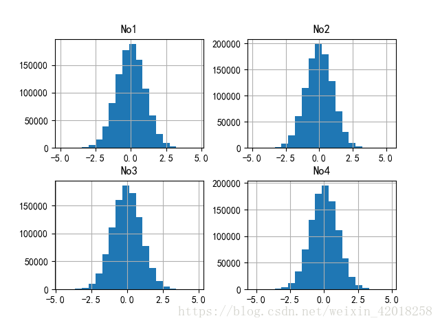
hist,bar 区别:
https://zhidao.baidu.com/question/142311366.html
hist是制作一个频率分布图,比如说把一个数据分成10个部分,每个部分的频率是多少。 就是大概看一下数据的分布。 bar是用来把你已经总结好的数据画出来,可以用来对比各个组的数据。 总之hist只是专门制作频率分布的,而bar的应用范围很广,你可以同时对比多个组,还可以更细的分组。你如果分好了数据,用bar也能做到hist的效果。
7.2.4 Excel文件数据
%time data[:100000].to_excel(filename+'.xlsx')
# Wall time: 22.3 s
%time pd.read_excel(filename+'.xlsx','Sheet1').cumsum().plot()
# Wall time: 11.4 s
对生成的文件进行检查发现, DataFrem与HDFStore 相结合是最为紧凑的备方法(使用本章后面介绍的压缩可以进一步加强这 一优势)。同样的数据量如果用 csv 文件(即文本文件)存储。文件尺寸会更大。 这是使用 csv 文件的性能较低的原因之一 , 另一
个原因是它们只是“一般的文本文件”
7.3 PyTables的快速I/O
PyTables是Python和HDF5数据库/文件标准的结合。它专门为优化I/O操作的性能、最大限度的利用可用硬件而设计。该库的导入名称为tables。在内存分析方面PyTables与pandas类似,并不是用于代替数据库的,而是引入某些功能,进一步弥补不足。例如,PyTables数据库可用有许多表,且支持压缩和索引,以及表的重要查询。此外,它可以高效的存储Numpy数组,并且具有自己独特的类数组数据结构。
7.3.1 使用表
import numpy as np
import tables as tb
import datetime as dt
import matplotlib.pyplot as plt
filename=path+'tab.h5'
h5=tb.open_file(filename,'w')
rows=2000000
row_des={
    'Date':tb.StringCol(26,pos=1),
    'No1':tb.IntCol(pos=2),
    'No2':tb.IntCol(pos=3),
    'No3':tb.Float64Col(pos=4),
    'No4':tb.Float64Col(pos=5)
}
# 创建表格时,我们选择无压缩。后续的例子将加入压缩
filters = tb.Filters(complevel=0)  # no compression
tab = h5.create_table('/', 'ints_floats', row_des,
                      title='Integers and Floats',
                      expectedrows=rows, filters=filters)
tab
# /ints_floats (Table(0,)) 'Integers and Floats'
#   description := {
#   "Date": StringCol(itemsize=26, shape=(), dflt=b'', pos=0),
#   "No1": Int32Col(shape=(), dflt=0, pos=1),
#   "No2": Int32Col(shape=(), dflt=0, pos=2),
#   "No3": Float64Col(shape=(), dflt=0.0, pos=3),
#   "No4": Float64Col(shape=(), dflt=0.0, pos=4)}
#   byteorder := 'little'
#   chunkshape := (2621,)


pointer = tab.row
ran_int=np.random.randint(0,10000,size=(rows,2))
ran_flo=np.random.standard_normal((rows,2)).round(5)
%%time
for i in range(rows):
    pointer['Date']=dt.datetime.now()
    pointer['No1']=ran_int[i,0]
    pointer['No2']=ran_int[i,1]
    pointer['No3']=ran_flo[i,0]
    pointer['No4']=ran_flo[i,1]
    pointer.append()
    # this appends the data and move the pointer one row forward
tab.flush()  # 提交
# Wall time: 12.2 s

tab
# /ints_floats (Table(2000000,)) 'Integers and Floats'
#   description := {
#   "Date": StringCol(itemsize=26, shape=(), dflt=b'', pos=0),
#   "No1": Int32Col(shape=(), dflt=0, pos=1),
#   "No2": Int32Col(shape=(), dflt=0, pos=2),
#   "No3": Float64Col(shape=(), dflt=0.0, pos=3),
#   "No4": Float64Col(shape=(), dflt=0.0, pos=4)}
#   byteorder := 'little'
#   chunkshape := (2621,)

# 使用NumPy结构数组, 可以更高性能、更Python风格的方式实现相同结果
dty = np.dtype([('Date', 'S26'), ('No1', '), ('No2', '), ('No3', '), ('No4', ')])
sarray = np.zeros(len(ran_int), dtype=dty)
sarray

%%time
sarray['Date']=dt.datetime.now()
sarray['No1']=ran_int[:,0]
sarray['No2']=ran_int[:,1]
sarray['No3']=ran_flo[:,0]
sarray['No4']=ran_flo[:,1]
# Wall time: 96 ms

# 整个数据集现在都保存在结构数组中,表的创建归结为如下几行代码。注意,行描述不再需要;PyTables使用NumPy dtype代替:
%%time
h5.create_table('/', 'ints_floats_from_array', sarray,
                title='Integers and Floats',
                expectedrows=rows, filters=filters)
# Wall time: 126 ms
#
# /ints_floats_from_array (Table(2000000,)) 'Integers and Floats'
#   description := {
#   "Date": StringCol(itemsize=26, shape=(), dflt=b'', pos=0),
#   "No1": Int32Col(shape=(), dflt=0, pos=1),
#   "No2": Int32Col(shape=(), dflt=0, pos=2),
#   "No3": Float64Col(shape=(), dflt=0.0, pos=3),
#   "No4": Float64Col(shape=(), dflt=0.0, pos=4)}
#   byteorder := 'little'
#   chunkshape := (2621,)

# 这种方法的速度比前一种方法快了一个数量级, 以更少的代码实现了相同的结果
h5
# File(filename=E:/Projects/DEMO/Py/MyPyTest/MyPyTest/python_for_finance/data/tab.h5, title='', mode='w', root_uep='/', filters=Filters(complevel=0, shuffle=False, fletcher32=False, least_significant_digit=None))
# / (RootGroup) ''
# /ints_floats (Table(0,)) 'Integers and Floats'
#   description := {
#   "Date": StringCol(itemsize=26, shape=(), dflt=b'', pos=0),
#   "No1": Int32Col(shape=(), dflt=0, pos=1),
#   "No2": Int32Col(shape=(), dflt=0, pos=2),
#   "No3": Float64Col(shape=(), dflt=0.0, pos=3),
#   "No4": Float64Col(shape=(), dflt=0.0, pos=4)}
#   byteorder := 'little'
#   chunkshape := (2621,)
# /ints_floats_from_array (Table(2000000,)) 'Integers and Floats'
#   description := {
#   "Date": StringCol(itemsize=26, shape=(), dflt=b'', pos=0),
#   "No1": Int32Col(shape=(), dflt=0, pos=1),
#   "No2": Int32Col(shape=(), dflt=0, pos=2),
#   "No3": Float64Col(shape=(), dflt=0.0, pos=3),
#   "No4": Float64Col(shape=(), dflt=0.0, pos=4)}
#   byteorder := 'little'
#   chunkshape := (2621,)

# 现在可以删除重复的表, 因为已经不再需要
h5.remove_node('/','ints_floats_from_array')
# 表(Table)对象的表现在切片时的表现与典型的Pthon和NumPy对象类似
tab[:3]
# array([(b'2018-06-28 15:58:53.056742', 5346, 1485, -0.20095, -1.31293),
#        (b'2018-06-28 15:58:53.056742', 9161, 9732, -0.07978, -0.66802),
#        (b'2018-06-28 15:58:53.056742', 4935, 5664,  0.17463,  0.56233)],
#       dtype=[('Date', 'S26'), ('No1', '
tab[:4]['No4']
# array([-1.31293, -0.66802,  0.56233,  0.42158])
%time np.sum(tab[:]['No3'])
# Wall time: 114 ms
# -1692.7833899999991
%time np.sum(np.sqrt(tab[:]['No1']))
# Wall time: 135 ms
# 133364497.15106584

# 数据直方图
%%time
plt.hist(tab[:]['No3'], bins=30)
plt.grid(True)
print(len(tab[:]['No3']))
# 2000000
# Wall time: 505 ms 
# 查询结果的散点图
%%time
res=np.array([(row['No3'],row['No4']) for row in tab.where('((No3<-0.5)|(No3>0.5))&((No4<-1)|(No4>1))')])[::100]
plt.plot(res.T[0],res.T[1],'ro')
plt.grid(True)
# Wall time: 472 ms
# pandas 和 PyTable 都能处理复杂的类 SQL 查询及选择 。 它们都对这些操作的速度进行了优化 。

%%time
values=tab.cols.No3[:]
print("Max %18.3f" % values.max())
print("Ave %18.3f" % values.mean())
print("Min %18.3f" % values.min())
print("Std %18.3f" % values.std())
# Max              4.953
# Ave             -0.001
# Min             -5.162
# Std              1.000
# Wall time: 99 ms

%%time
results=[(row['No1'],row['No2']) for row in tab.where('((No1>9800)|(No1<200))&((No2>4500)&(No2<5500))')]
for res in results[:4]:
    print(res)
# (9921, 4993)
# (137, 4994)
# (165, 4878)
# (9832, 5033)
# Wall time: 107 ms

%%time
results=[(row['No1'],row['No2']) for row in tab.where('(No1==1234)&(No2>9776)')]
for res in results[:4]:
    print(res)
# (1234, 9840)
# (1234, 9825)
# (1234, 9854)
# (1234, 9927)
# Wall time: 86 ms
7.3.2 使用压缩表
使用 PyTables 的主要优势之一是压缩方法。 使用压缩不仅能节约磁盘空间, 还能改善I/O 操作的性能。这是如何实现的?当 I/O成为瓶颈而CPU 能够快速(解)压缩数据时,使用压缩对速度有正面的净效应。
filename=path+'tab.h5c'
h5c = tb.open_file(filename, 'w')
filters = tb.Filters(complevel=4, complib='blosc')
tabc = h5c.create_table('/', 'ints_floats', sarray, title='Integers and Floats', expectedrows=rows, filters=filters)

%%time
res=np.array([(row['No3'],row['No4']) for row in tabc.where('((No3<-0.5)|(No3>0.5))&((No4<-1)|(No4>1))')])[::100]
# Wall time: 530 ms
# 生成包含原始数据的表并在上面进行分析比未压缩的表稍慢

%time arr_non=tab.read()
# Wall time: 104 ms

%time arr_com=tabc.read()
# Wall time: 200 ms

# 这种方法花的时间确实比以前长。 但是 ,压缩率大约为20% ,节约80%磁盘间。对于备份历程或者服务器之间甚至数据中心之间交换大数据集可能很重要

h5c.close()
7.3.3 使用数组
%%time
arr_int = h5.create_array('/', 'integers', ran_int)
arr_flo = h5.create_array('/', 'floats', ran_flo)
# Wall time: 195 ms
# 现在库中有3个对象一表和两个数组:
h5
# File(filename=E:/Projects/python_for_finance/data/tab.h5, title='', mode='w', root_uep='/', filters=Filters(complevel=0, shuffle=False, fletcher32=False, least_significant_digit=None))
# / (RootGroup) ''
# /floats (Array(2000000, 2)) ''
#   atom := Float64Atom(shape=(), dflt=0.0)
#   maindim := 0
#   flavor := 'numpy'
#   byteorder := 'little'
#   chunkshape := None
# /integers (Array(2000000, 2)) ''
#   atom := Int32Atom(shape=(), dflt=0)
#   maindim := 0
#   flavor := 'numpy'
#   byteorder := 'little'
#   chunkshape := None
# /ints_floats (Table(2000000,)) 'Integers and Floats'
#   description := {
#   "Date": StringCol(itemsize=26, shape=(), dflt=b'', pos=0),
#   "No1": Int32Col(shape=(), dflt=0, pos=1),
#   "No2": Int32Col(shape=(), dflt=0, pos=2),
#   "No3": Float64Col(shape=(), dflt=0.0, pos=3),
#   "No4": Float64Col(shape=(), dflt=0.0, pos=4)}
#   byteorder := 'little'
#   chunkshape := (2621,)
h5.close()
基于 HDF5 的数据存储
HDF5 数据库(文件)格式是结构化数值和金融数据的强大替代方案,例如可以用它代替关系数据库。在使用PyTbles时单位访问或者结合pandas的能力, 都可以得到硬件所能支持的最高I/0性能。
7.3.4 内存外计算
filename=path+'array.h5'
h5=tb.open_file(filename,'w')
n=1000
ear = h5.create_earray(h5.root, 'ear', atom=tb.Float16Atom(), shape=(0, n))
%%time
rand=np.random.standard_normal((n,n))
for i in range(750):
    ear.append(rand)
ear.flush()

out = h5.create_earray(h5.root, 'out', atom=tb.Float16Atom(), shape=(0, n))
expr = tb.Expr('3*sin(ear)+sqrt(abs(ear))')
expr.set_output(out, append_mode=True)
%time expr.eval()
# Wall time: 9.81 s
#
# /out (EArray(750000, 1000)) ''
#   atom := Float16Atom(shape=(), dflt=0.0)
#   maindim := 0
#   flavor := 'numpy'
#   byteorder := 'little'
#   chunkshape := (32, 1000)

out[0,:10]
# array([-0.62988281,  0.2286377 ,  0.77636719,  4.06640625,  2.29296875,
#         2.203125  ,  3.90234375, -1.76464844,  0.11865234, -1.75292969], dtype=float16)

%time imarray=ear.read()
# Wall time: 1.56 s

import numexpr as ne
expr='3*sin(ear)+sqrt(abs(ear))'
ne.set_num_threads(16)
%time ne.evaluate(expr)[0,:10]
# Wall time: 15.4 s
#
# array([-0.62968171,  0.22863297,  0.77652252,  4.06454182,  2.29324198,
#         2.20375967,  3.9031148 , -1.76456189,  0.11864985, -1.75273955], dtype=float32)

h5.close()
end