Physically Based Rendering——史上最容易理解的BRDF中D函数NDF的中文资料

转存失败重新上传取消转存失败重新上传取消

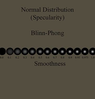
为了吸引读者眼球，开头引用了虚幻文档里的粗糙度变化的图，让大家对粗糙度有个直观的概念。

粗糙度决定了D函数的分布，一般粗糙度是D函数的方差

本文假定读者已经对PBR即Physcially Based Rendering 基于物理的渲染有了初步的了解，对于PBR的入门有很多文章都介绍的不错。

本文针对想再了解下BRDF双向反射分布函数里的推导与内容的读者，是我自己学习BRDF的笔记

这篇文章主要介绍BRDF里的法线分布函数D函数的各种算法于思想

D函数描述了微表面有多少比例的微表面的朝向是可以把光反射到眼睛的。

之前我的博客 手推系列——直观理解推导Physically Based Rendering 的BRDF公式之微表面法线分布函数NDF

用暴力的方式展示了NDF的概念和大题样子

假设高度图是平均分布，那么计算的NDF样子

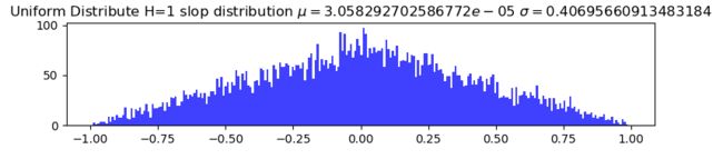
假设高度图是高斯分布，那么计算的NDF样子

下面介绍一些流行的NDF的公式和思想

Torrance Sparrow D函数 或者 高斯分布

来自与论文 Theory for Off-Specular Reflection From Roughened Surfaces Author

考虑一个斜率分布是高斯分布的微表面，很明显朝向某个方向的微表面的比例也满足高斯分布。这就是著名的高斯分布D函数，就是Torrance and Sparrow的BRDF模型里用的D函数，原始论文是这么写的

Blinn说的Torrance and Sparrow D函数是这样的

看起来这个样子

#Blinn说的Torrance and Sparrow 高斯分布D函数  from cook paper
def TorranceSparrow_D(roughness, theta):
    c = 1
    return c * np.exp(-np.power(theta/roughness,2))

其中b,c 是常数，b是微表面法线方向为宏观表面时候法线方向的时候的概率，c明显是正态分布的标准差的导数。

a是微表面法线和宏观法线的夹角。现在一般流行叫做 NoH

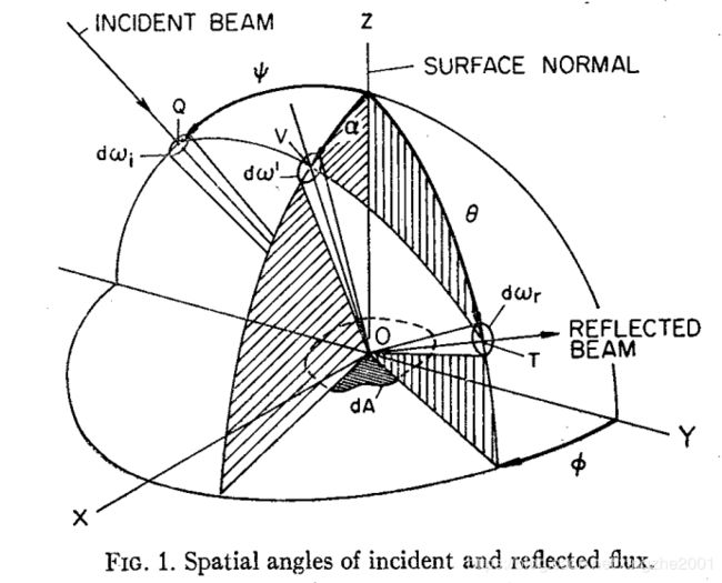
上图来自于 Theory for Off-Specular Reflection From Roughened Surfaces Author: K. E. Torrance and E. M. Sparrow

Jordan给出的渲染效果是这样的

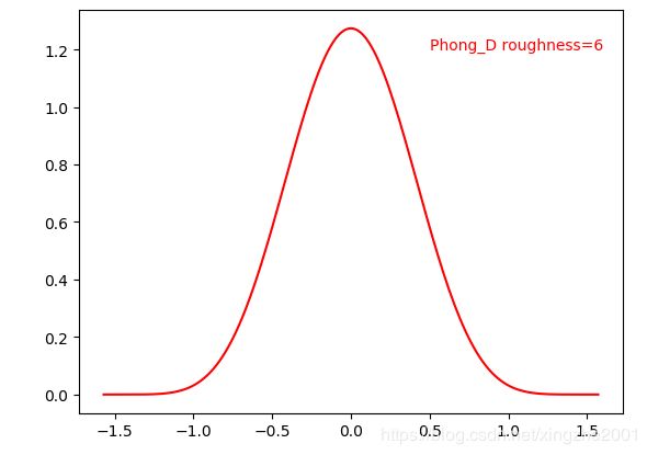
Phong模型 

公式来自于Blinn的 Models of light reflection for computer synthesized pictures

 

代码如下

#Phong Mode from blinn paper, normallized with ggx paper
def Phong_D(roughness, theta):
    return (roughness + 2)/(2*np.pi)*np.power(np.cos(theta), roughness)

略有改动，GGX论文对他进行了缩放，不影响形状

Jordan给出的渲染效果是这样的

Beckmann分布

原始论文在Beckmann的书里，找不到他的书的下载，Cook的论文里这么给出的

代码如下

#Beckmann D分布，from cook paper, ggx paper
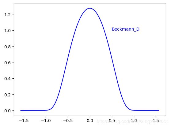
def Beckmann_D(roughness, theta):
    cos_theta = np.cos(theta)
    tan_theta = np.tan(theta)

    return np.exp(-np.power(tan_theta/roughness,2))/(np.pi*roughness*roughness*np.power(cos_theta,4))

长这个样子

Cook 在他的论文里 A reflectance model for computer graphics 很喜欢用。他的论文有人翻译https://blog.uwa4d.com/archives/Study_PBR.html 

Beckmann的公式怎么推出来的我没找到资料，不过他比高斯模型好，没有奇怪的常数，所有参数都有物理意义

Jordan给出的渲染图

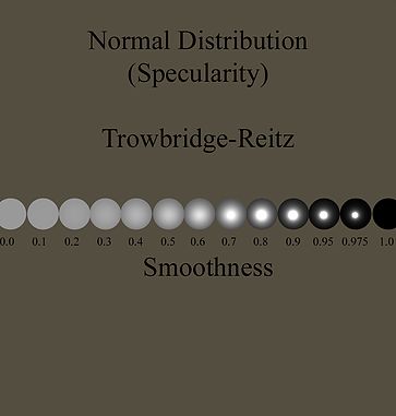
TrowbridgeReitz 模型

来自于 TrowbridgeReitz 的论文 Average irregularity representation of a rough surface for ray reflection

该模型和前面将的不同的是，微表面不是一个完美反射的平面镜面，而是一个完美反射的椭球面。因此微表面反射的光更加发散，高光拖尾也越长。

来自于Blinn的论文的公式

其实是一样的

代码如下

#Trowbridge and Reitz D分布，From blinn paper ellipsoids of revolution
def TrowbridgeReitz_D(roughness, theta):
        c = 1/np.pi/roughness/roughness
        return np.power(roughness*roughness/(np.power(np.cos(theta),2) * (roughness*roughness-1)+1),2)*c

形状是这样的

渲染效果如图

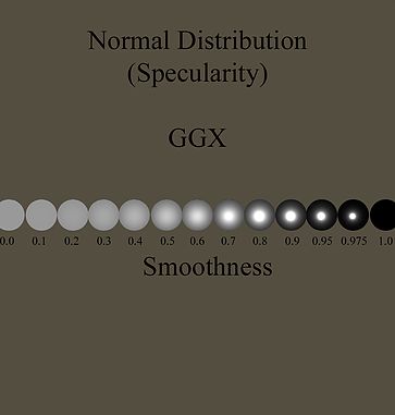
GGX 模型

现在用到最多的NDF函数，Unreal, Untiy都在使用。高光拖尾很美，算法模型和TrowbridgeReitz 类似。据他自己说和TrowbridgeReitz在数学上是等价的。

GGX的论文是 Microfacet Models for Refraction through Rough Surfaces

GGX D函数的论文 

 

GGX 是目前最流行的 

公式为

那个x相当于sign()

代码为

#GGX 分布 from ggx papaer
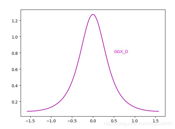
def GGX_D(roughness, theta):
    cos_theta = np.cos(theta)
    tan_theta = np.tan(theta)

    return roughness*roughness/(np.pi*np.power(cos_theta,4)*np.power(roughness*roughness + np.power(tan_theta,2),2))

函数图形为

渲染效果为

 

所有函数图形的比较为

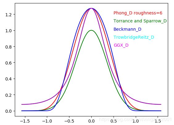
Torrance Sparrow高斯分布没有归一化

 

参考资料

• 学术界 Blinn论文 Models of Light Reflection for Computer Synthesized Pictures 比较了不少D函数。
• 工业界 Jordan Stevens 很多NDF的实现和比较 http://www.jordanstevenstechart.com/physically-based-rendering
• 著名的理解NDF的文章 How Is The NDF Really Defined? http://www.reedbeta.com/blog/hows-the-ndf-really-defined/
• 虚幻Brian karis的brdf参考 http://graphicrants.blogspot.com/2013/08/specular-brdf-reference.html

附录

所有NDF的代码和曲线代码

import matplotlib.pyplot as plt
import numpy as np
import scipy.stats as stats

#Phong Mode from blinn paper, normallized with ggx paper
def Phong_D(roughness, theta):
    return (roughness + 2)/(2*np.pi)*np.power(np.cos(theta), roughness)

#Blinn说的Torrance and Sparrow 高斯分布D函数  from cook paper
def TorranceSparrow_D(roughness, theta):
    c = 1
    return c * np.exp(-np.power(theta/roughness,2))

#Beckmann D分布，from cook paper, ggx paper
def Beckmann_D(roughness, theta):
    cos_theta = np.cos(theta)
    tan_theta = np.tan(theta)

    return np.exp(-np.power(tan_theta/roughness,2))/(np.pi*roughness*roughness*np.power(cos_theta,4))

#Trowbridge and Reitz D分布，From blinn paper ellipsoids of revolution
def TrowbridgeReitz_D(roughness, theta):
        c = 1/np.pi/roughness/roughness
        return np.power(roughness*roughness/(np.power(np.cos(theta),2) * (roughness*roughness-1)+1),2)*c

#GGX 分布 from ggx papaer
def GGX_D(roughness, theta):
    cos_theta = np.cos(theta)
    tan_theta = np.tan(theta)

    return roughness*roughness/(np.pi*np.power(cos_theta,4)*np.power(roughness*roughness + np.power(tan_theta,2),2))


theta=np.linspace(-np.pi*0.5,np.pi*0.5,180)
plt.plot(theta, Phong_D(6, theta), "r-")
plt.text(0.5,1.2,"Phong_D roughness=6",color="red")

plt.plot(theta, TorranceSparrow_D(0.5, theta), "g-")
plt.text(0.5,1.1,"Torrance and Sparrow_D",color="green")

plt.plot(theta, Beckmann_D(0.5, theta), "b-")
plt.text(0.5,1.0,"Beckmann_D",color="blue")

plt.plot(theta, TrowbridgeReitz_D(0.5, theta), "c-")
plt.text(0.5,0.9,"TrowbridgeReitz_D",color="cyan")

plt.plot(theta, GGX_D(0.5, theta), "m-")
plt.text(0.5,0.8,"GGX_D",color="magenta")
plt.show()