[Notes] Introduction to The Design and Analysis of Algorithms from Anany Levitin
[Notes] Introduction to The Design and Analysis of Algorithms from Anany Levitin
- Exercise solutions for 2nd edition
- 1. Introduction
- 1.1 What is an Algorithm?
- Greatest Common Divisor
- 1.2 Fundamentals of Algorithmic Problem Solving
- 1.3 Important Problem Types
- 1.4 Fundamental Data Structures
- 2. Fundamentals of the Analysis of Algorithm Efficiency
- 2.1 The Analysis Framework
- 2.2 Asymptotic Notations and Basic Efficiency Classes
- 2.3 Mathematical Analysis of Nonrecursive Algorithms
- 2.4 Mathematical Analysis of Recursive Algorithms
- 2.6 Empirical Analysis of Algorithms
- 3. Brute Force and Exhaustive Search
- 3.1 Selection Sort and Bubble Sort
- Selection Sort
- Bubble Sort
- 3.2 Sequential search and Brute-Force String Matching
- Sequential search
- Brute-Force String Matching
- 3.3 Closest-Pair Problem and Convex-Hull Problem
- Closest-Pair Problem
- Convex-Hull Problem
- 3.4 Exhaustive Search
- 3.5 Depth-First Search and Breadth-First Search
- Depth-First Search
- Breadth-First Search
- 4. Decrease-and-Conquer
- 4.1 Insertion Sort
- Exercises 4.1
- 4.2 Topological Sorting
- Algorithm 1:
- Algorithm 2:
- Exercises 4.2
- 4.3 Algorithms for Generating Combinatorial Objects
- Generating Permutations
- Generating Subsets
- Exercises 4.3
- 4.4 Decrease-by-a-Constant-Factor Algorithms
- Binary Search
- Josephus Problem
- Exercises 4.4
- 4.5 Variable-Size-Decrease Algorithms
- Computing a Median and the Selection Problem
- Interpolation Search
- Searching and Insertion in a Binary Search Tree
- The Game of Nim
- 5. Divide-and-Conquer
- 5.1 Mergesort
- Exercises 5.1
- 5.2 Quicksort
- 5.3 Binary Tree Traversals and Related Properties
- 5.4 Multiplication of Large Integers and Strassen’s Matrix Multiplication
- Multiplication of Large Integers
- Strassen’s Matrix Multiplication
- 5.5 The Closest-Pair and Convex-Hull Problems by Divide-and-Conquer
- The Closest-Pair Problem
- Convex-Hull Problem
- 6. Transform-and-Conquer
- 6.1 Presorting
- Exercises 6.1
- 6.2 Guassian Elimination
- 6.3 Balanced Search Trees
- AVL tree
- 2-3 Trees
- 6.4 Heaps and Heapsort
- Heapsort
- 6.5 Horner’s Rule and Binary Exponentiation
- Horner’s Rule
- Binary Exponentiation
- 6.6 Problem Reduction
- Computing the Least Common Multiple
- Counting Paths in a Graph
- Reduction of Optimization Problems
- Linear Programming
- Reduction to Graph Problems
- 7. Space and Time Trade-Offs
- 7.1 Sorting by counting
- comparison-counting sort
- distribution counting
- 7.2 Input Enhancement in String Matching
- Horspool's Algorithm
- Boyer-Moore Algorithm
- 7.3 Hashing
- Open Hashing (Separate Chaining)
- Closed Hashing (Open Addressing)
- 7.4 B-trees
- 8. Dynamic Programming
- 8.1 Three Basic Examples
- 8.2 The Knapsack Problem and Memory Functions
- The Knapsack Problem
- Memory Functions
Exercise solutions for 2nd edition
2nd Edition solutions
1. Introduction
1.1 What is an Algorithm?
Important points:
- The non-ambiguity requirement for each step of an algorithm cannot be comprimised.
- The range of inputs for which an algorithm works has to be specified carefully.
- The same algorithm can be represented in several different ways.
- There must exist several algorithms for solving the same problem.
- Algorithms for the same problem can be based on very different ideas and can solve the problem with dramatically different speeds.
Greatest Common Divisor
Method 1:
Euclid's algorithm: for computing gcd(m, n)
Step 1: If n=0, return the value of m as the answer and stop; otherwise, proceed to Step2.
Step 2: Divide m by n and assign the value of the reminder to r.
Step 3: Assign the value of n to m and the value of r to n. Go to Step1.
ALGORITHM Euclid(m, n)
//Computes gcd(m, n) by Euclid's algorithm
//Input: Two nonnegative, not-both-zero integers m and n
//Output: Greatest common divisor of m and n
while n ≠ 0 do
  r ← m mod n
  m ← n
  n ← r
return m
Proof of Euclid’s algorithm: for computing gcd(m, n)
Method 2:
Consecutive integer checking algorithm for computing gcd(m, n)
Step 1: Assign the value of min{m, n} to t.
Step 2: Divide m by t. If the remainder of this division is 0. go to Step3; otherwise, go to Step4.
Step 3: Divide n by t. If the remainder of this division is 0, return the value of t as the answer and stop; otherwise, proceed to Step4.
Step 4: Decrease the value of t by 1. Go to Step2.
This algorithm in the form presented, doesn’t work correctly when one of its input numbers is zero. It also underlines that it’s important to specify the set of an algorithm’s inputs explicitly and carefully.
Method 3:
Middle-school procedure for computing gcd(m, n)
Step 1: Find the prime factors of m.
Step 2: Find the prime factors of n.
Step 3: Identify all the common factors in the two prime expansions found in Step 1 and 2. (If p is a common factor occurring q1 and q2 times in m and n, respectively, it should be  repeated min{q1, q2} times.)
Step 4: Compute the product of all the common factors and return it as the greatest common divisor of the numbers given.
Prime factors in Step 1 and 2 is not unambiguous. Also, Step 3 is not straightforward which makes Method 3 an unqualified algorithm. This is why Sieve of Eratosthenes needs to be introduced (generate consecutive primes not exceeding any given integer n > 1).
Sieve of Eratosthenes (Overview and Pseudocode part)
ALGORITHM Sieve(n)
//Implements the sieve of Eratosthenes
//Input: A positive integer n > 1
//Ouput: Array L of all prime numbers less than or equal to n
for p <- 2 to n do A[p] <- p
for p <-2 to floor(sqrt(n)) do
	if A[p] not equal to 0 //p hasn't been eliminated on previous passes
		j <- p * p
		while j <= n do
			A[j] <- 0  //mark elements as eliminated
			j <- j + p
//copy the remaining elements of A to array L of the primes
i <- 0
for p <- 2 to n do
	if A[p] not equal to 0
		L[i] <- A[p]
		i <- i + 1
return L
Q: What is the largest number p whose multiples can still remain on the list to make further iterations of the algorithm necessary?
A: If p is a number whose multiples are being eliminated on the current pass, then the first multiple we should consider is p 2 p^2 p2 because all its smaller multiples 2 p , … , ( p − 1 ) p 2p,\dots,(p-1)p 2p,…,(p−1)p have been eliminated on earlier passes through the list. Obviously, p 2 p^2 p2 should not be greater than n n n.
Special care needs to be exercised if one or both input numbers are equal to 1: because mathematicians do not consider 1 to be a prime number, strictly speaking, the method does not work for such inputs.
1.2 Fundamentals of Algorithmic Problem Solving
-
Understanding the Problem:
Read the problem’s description carefully and ask questions if you have any doubts about the problem, do a few small examples by hand, think about special cases, and ask questions again if needed.
An input to an algorithm specifies an instance of the problem the algorithm solves. If you fail to do this step, your algorithm may work correctly for a majority of inputs but crash on some “boundary” value. Remember a correct algorithm is not one that works most of the time, but one that works correctly for all legitimate inputs.
-
Ascertaining the Capabilities of the Computational Device:
RAM (random-access machine): instructions are executed one after another, one operation at a time, use sequential algorithms.
New computers: execute operations concurrently, use parallel algorithms.
Also, consider the speed and amount of memory the algorithm would take for different situations.
-
Choosing between Exact and Approximate Problem Solving
-
Algorithm Design Techniques
-
Designing an Algorithm and Data Structures
-
Methods of Specifying an Algorithm: natural language vs pseudocode
-
Proving an Algorithm’s Correctness: the algorithm yields a required result for every legitimate input in a finite amount of time.
A common technique for proving correctness is to use mathematical induction because an algorithm’s iterations provide a natural sequence of steps needed for such proofs.
For an approximation algorithm, we usually would like to show that the error produced by the algorithm does not exceed a predefined limit.
-
Analyzing an Algorithm: time and space efficiency, simplicity, generality.
“A designer knows he has arrived at perfection not when there is no longer anything to add, but when there is no longer anything to take away.” —— Antoine de Saint-Exupery
-
Coding an algorithm
As a rule, a good algorithm is a result of repeated effort and rework.
1.3 Important Problem Types
The important problem types are sorting, searching, string processing, graph problems, combinatorial problems, geometric problems, and numerical problems.
-
Sorting
Rearrange the items of a given list in nondecreasing order according to a key.Although some algorithms are indeed better than others, there is no algorithm that would be the best solution in all situations.
A sorting algorithm is called stable if it preserves the relative order of any two equal elements in its input, in-place if it does not require extra memory.
1.4 Fundamental Data Structures
Algorithms operate on data. This makes the issue of data structuring critical for efficient algorithmic problem solving. The most important elementary data structures are the array and the linked list. They are used for representing more abstract data structures such as the list, the stack, the queue/ priority queue (better implementation is based on an ingenious data structure called the heap), the graph (via its adjacency matrix or adjacency lists), the binary tree, and the set.
-
Graph
A graph with every pair of its vertices connected by an edge is called complete. A graph with relatively few possible edges missing is called dense; a graph with few edges relative to the number of its vertices is called sparse. -
Trees
A tree is a connected acyclic graph. A graph that has no cycles but is not necessarily connected is called a forest: each of its connected components is a tree.The number of edges in a tree is always one less than the number of its vertices:|E| = |V| - 1. This property is necessary but not sufficient for a graph to be a tree. However, for connected graphs it is sufficient and hence provides a convenient way of checking whether a connected graph has a cycle.
Ordered trees, ex. binary search trees. The efficiency of most important algorithms for binary search trees and their extensions depends on the tree’s height. Therefore, the following inequalities for the height h of a binary tree with n nodes are especially important for analysis of such algorithms: ⌊ log 2 n ⌋ ≤ h ≤ n − 1 \lfloor\log_2{n}\rfloor \leq h \leq n - 1 ⌊log2n⌋≤h≤n−1
-
Sets
Representation of sets can be: a bit vector and list structure.
An abstract collection of objects with several operations that can be performed on them is called an abstract data type (ADT). The list, the stack, the queue, the priority queue, and the dictionary are important examples of abstract data types. Modern object-oriented languages support implementation of ADTs by means of classes.
2. Fundamentals of the Analysis of Algorithm Efficiency
Running time and memory space.
2.1 The Analysis Framework
The research experience has shown that for most problems, we can achieve much more spectacular progress in speed than in space.
-
Measuring an Input’s Size
When measuring input size for algorithms solving problems such as checking primality of a positive integer n. Here, the input is just one number, and it is this number’s magnitude that determines the input size. In such situations, it is preferable to measure size by the number b of bits in the n’s binary representation: b = ⌊ log 2 n ⌋ + 1 b = \lfloor\log_2{n}\rfloor + 1 b=⌊log2n⌋+1 -
Units for Measuring Running Time
The thing to do is to identify the most important operation of the algorithm, called the basic operation, the operation contributing the most to the total running time, and compute the number of times the basic operation is executed.Algorithms for mathematical problems typically involve some or all of the four arithmetical operations: addition, subtraction, multiplication and division. Of the four, the most time-consuming operation is division, followed by multiplication and then addition and subtraction, with the last two usually considered together.
The established framework for the analysis of an algorithm’s time efficiency suggests measuring it by counting the number of times the algorithm’s basic operation is executed on inputs of size n.
-
Orders of Growth
logan = logab * logbnAlgorithms that require an exponential number of operations are practical for solving only problems of very small sizes.
-
Worst-Case, Best-Case, and Average-Case Efficiencies
If the best-case efficiency of an algorithm is unsatisfactory, we can immediately discard it without further analysis.The direct approach for investigating average-case efficiency involves dividing all instances of size n into several classes so that for each instance of the class the number of times the algorithm’s basic operation is executed is the same. Then a probability distribution of inputs is obtained or assumed so that the expected value of the basic operation’s count can be found.
Amortized efficiency.
Space efficiency is measured by counting the number of extra memory units consumed by the algorithm.
The efficiencies of some algorithms may differ significantly for inputs of the same size. For such algorithms, we need to distinguish between the worst-case, average-case, and best-case efficiencies.
2.2 Asymptotic Notations and Basic Efficiency Classes
-
O-notation
O(g(n)) is the set of all functions with a lower or same order of growth as g(n) (to within a constant multiple, as n goes to infinity).Definition: A function t(n) is said to be in O(g(n)), denoted t(n) ∈ O(g(n)), if t(n) is bounded above by some constant multiple of g(n) for all large n, i.e., if there exist some positive constant c and some nonnegative integer n0 such that t(n) ≤ cg(n) for all n ≥ n0
-
Ω-notation
Ω(g(n)) is the set of all functions with a higher or same order of growth as g(n) (to within a constant multiple, as n goes to infinity).Definition: A function t(n) is said to be in Ω(g(n)), denoted t(n) ∈ Ω(g(n)), if t(n) is bounded below by some constant multiple of g(n) for all large n, i.e., if there exist some positive constant c and some nonnegative integer n0 such that t(n) ≥ cg(n) for all n ≥ n0
-
Θ-notation
Θ(g(n)) is the set of all functions with the same order of growth as g(n) (to within a constant multiple, as n goes to infinity).Definition: A function t(n) is said to be in Θ(g(n)), denoted t(n) ∈ Θ(g(n)), if t(n) is bounded both above and below by some constant multiples of g(n) for all large n, i.e., if there exist some positive constant c1 and c2 and some nonnegative integer n0 such that c2g(n) ≤ t(n) ≤ c1g(n) for all n ≥ n0.
-
Useful Property Involving the Asymptotic Notations
If t1(n) ∈ O(g1(n)) and t2(n) ∈ O(g2(n)), then t1(n) + t2(n) ∈ O(max{g1(n), g2(n)}) (also true for other two notations).
![[Notes] Introduction to The Design and Analysis of Algorithms from Anany Levitin_第1张图片](http://img.e-com-net.com/image/info8/367f81720347498ca56cb971929171ac.jpg)
L’Hôpital’s rule:
![[Notes] Introduction to The Design and Analysis of Algorithms from Anany Levitin_第2张图片](http://img.e-com-net.com/image/info8/618fe01a14ab4fb69440607d442e801d.jpg)
Stirling’s Formula:
![[Notes] Introduction to The Design and Analysis of Algorithms from Anany Levitin_第3张图片](http://img.e-com-net.com/image/info8/262843fbef444a86b6b64b51ffdfd996.jpg)
-
Basic asymptotic efficiency classes
![[Notes] Introduction to The Design and Analysis of Algorithms from Anany Levitin_第4张图片](http://img.e-com-net.com/image/info8/3854f03da05549d887c38e3b0aa3fb42.jpg)
2.3 Mathematical Analysis of Nonrecursive Algorithms
-
Decide on parameter (or parameters) n indicating an input’s size.
-
Identify the algorithm’s basic operation. (As a rule, it is located in the inner most loop.)
-
Check whether the number of times the basic operation is executed depends only on the size of an input. If it also depends on some additional property, the worst-case, average-case, and, if necessary, best-case efficiencies have to be investigated separately.
-
Set up a sum expressing the number of times the algorithm’s basic operation is executed.
-
Using standard formulas and rules of sum manipulation, either find a closed-form formula for the count or, at the very least, establish its order of growth.
Mathematical Analysis of Nonrecursive Algorithms
2.4 Mathematical Analysis of Recursive Algorithms
- Method of backward substitutions
- General Plan for Analyzing the Time Efficiency of Recursive Algorithms
- Decide on a parameter (or parameters) indicating an input’s size.
- Identify the algorithm’s basic operation.
- Check whether the number of times the basic operation is executed can vary on different inputs of the same size; if it can, the worst-case, average-case, and best-case efficiencies must be investigated separately.
- Set up a recurrence relation, with an appropriate initial condition, for the number of times the basic operation is executed.
- Solve the recurrence or, at least, ascertain the order of growth of its solution.
-
Tower of Hanoi
To move n > 1 disks from peg 1 to peg 3 (with peg 2 as auxiliary), we first move recursively n − 1 disks from peg 1 to peg 2 (with peg 3 as auxiliary), then move the largest disk directly from peg 1 to peg 3, and, finally, move recursively n − 1 disks from peg 2 to peg 3 (using peg 1 as auxiliary). Of course, if n = 1, we simply move the single disk directly from the source peg to the destination peg.
![[Notes] Introduction to The Design and Analysis of Algorithms from Anany Levitin_第5张图片](http://img.e-com-net.com/image/info8/a4219bdf3b6541b5b88f8f52ecca7134.jpg)
One should be careful with recursive algorithms because their succinctness may mask their inefficiency. -
BinRec(n): smoothness rule
ALGORITHM     BinRec(n)
//Input: A positive decimal integer n
//Output: The number of binary digits in n’s binary representation
if n = 1 return 1
else return BinRec(floor(n/2)) + 1
2.6 Empirical Analysis of Algorithms
- General Plan for the Empirical Analysis of Algorithm Time Efficiency
- Understand the experiment’s purpose.
- Decide on the efficiency metric M to be measured and the measurement unit (an operation count vs. a time unit).
- Decide on characteristics of the input sample (its range, size, and so on).
- Prepare a program implementing the algorithm (or algorithms) for the experimentation.
- Generate a sample of inputs.
- Run the algorithm (or algorithms) on the sample’s inputs and record the data observed.
- Analyze the data obtained.
- linear congruential method
ALGORITHM     Random(n, m, seed, a, b)
//Generates a sequence of n pseudorandom numbers according to the linear congruential method
//Input: A positive integer n and positive integer parameters m, seed, a, b
//Output: A sequence r1,...,rn of n pseudorandom integers uniformly distributed among integer values between 0 and m − 1 //Note: Pseudorandom numbers between 0 and 1 can be obtained by treating the integers generated as digits after the decimal point

r0 ← seed
for i ← 1 to n do
	ri ← (a ∗ ri−1 + b) mod m
The simplicity of this pseudocode is misleading because the devil lies in the details of choosing the algorithm’s parameters. Here is a partial list of recommendations based on the results of a sophisticated mathematical analysis (see [KnuII, pp. 184–185] for details): seed may be chosen arbitrarily and is often set to the current date and time; m should be large and may be conveniently taken as 2w, where w is the computer’s word size; a should be selected as an integer between 0.01m and 0.99m with no particular pattern in its digits but such that a mod 8 = 5; and the value of b can be chosen as 1.
3. Brute Force and Exhaustive Search
Brute force is a straightforward approach to solving a problem, usually directly based on the problem statement and definitions of the concepts involved.
3.1 Selection Sort and Bubble Sort
Selection Sort
We start selection sort by scanning the entire given list to find its smallest element and exchange it with the first element, putting the smallest element in its final position in the sorted list. Then we scan the list, starting with the second element, to find the smallest among the last n − 1 n − 1 n−1 elements and exchange it with the second element, putting the second smallest element in its final position. After n − 1 n − 1 n−1 passes, the list is sorted.
ALGORITHM SelectionSort(A[0..n − 1])
//Sorts a given array by selection sort
//Input: An array A[0..n − 1] of orderable elements
//Output: Array A[0..n − 1] sorted in nondecreasing order
for i ← 0 to n − 2 do
	min ← i
	for j ← i + 1 to n − 1 do
		if A[j] < A[min]
			min ← j
	swap A[i] and A[min]
The basic operation is the key comparison A [ j ] < A [ m i n ] A[j] < A[min] A[j]<A[min]. The number of times it is executed depends only on the array size n n n and is given by the following sum: C ( n ) = ∑ i = 0 n − 2 ∑ j = i + 1 n − 1 1 = ∑ i = 0 n − 2 ( n − 1 − i ) = ( n − 1 ) n 2 C(n)=\sum^{n-2}_{i=0}\sum^{n-1}_{j=i+1} 1 = \sum^{n-2}_{i=0}(n-1-i)={(n-1)n \over 2} C(n)=i=0∑n−2j=i+1∑n−11=i=0∑n−2(n−1−i)=2(n−1)n
Selection sort is a Θ ( n 2 ) \Theta(n^2) Θ(n2) algorithm on all inputs. Note, however, that the number of key swaps is only Θ ( n ) \Theta(n) Θ(n), or, more precisely, n − 1 n − 1 n−1 (one for each repetition of the i i i loop). This property distinguishes selection sort positively from many other sorting algorithms.
Bubble Sort
Another brute-force application to the sorting problem is to compare adjacent elements of the list and exchange them if they are out of order. By doing it repeatedly, we end up “bubbling up” the largest element to the last position on the list. The next pass bubbles up the second largest element, and so on, until after n − 1 n − 1 n−1 passes the list is sorted.
ALGORITHM BubbleSort(A[0..n − 1])
//Sorts a given array by bubble sort
//Input: An array A[0..n − 1] of orderable elements
//Output: Array A[0..n − 1] sorted in nondecreasing order
for i ← 0 to n − 2 do
	for j ← 0 to n − 2 − i do
		if A[j + 1] < A[j]
			swap A[j] and A[j + 1]
The number of key comparisons:
: C ( n ) = ∑ i = 0 n − 2 ∑ j = 0 n − 2 − i 1 = ∑ i = 0 n − 2 ( n − 1 − i ) = ( n − 1 ) n 2 ∈ Θ ( n 2 ) C(n)=\sum^{n-2}_{i=0}\sum^{n-2-i}_{j=0} 1 = \sum^{n-2}_{i=0}(n-1-i)={(n-1)n \over 2} \in \Theta(n^2) C(n)=i=0∑n−2j=0∑n−2−i1=i=0∑n−2(n−1−i)=2(n−1)n∈Θ(n2)
The number of key swaps, however, depends on the input. In the worst case of decreasing arrays, it is the same as the number of key comparisons:
S w o r s t ( n ) = C ( n ) = 1 + ⋯ + ( n − 1 ) = ( n − 1 ) n 2 ∈ Θ ( n 2 ) S_{worst}(n)=C(n)=1+\dots +(n-1)={(n-1)n \over 2}\in\Theta(n^2) Sworst(n)=C(n)=1+⋯+(n−1)=2(n−1)n∈Θ(n2)
A little trick: if a pass through the list makes no exchanges, the list has been sorted and we can stop the algorithm.Though the new version runs faster on some inputs, it is still in Θ ( n 2 ) \Theta(n^2) Θ(n2) in the worst and average cases.
Highlights:A first application of the brute-force approach often results in an algorithm that can be improved with a modest amount of effort.
3.2 Sequential search and Brute-Force String Matching
Sequential search
Trick1: if we append the search key to the end of the list, the search for the key will have to be successful, and therefore we can eliminate the end of list check altogether
ALGORITHM SequentialSearch2(A[0..n], K)
//Implements sequential search with a search key as a sentinel
//Input: An array A of n elements and a search key K
//Output: The index of the first element in A[0..n − 1] whose value is equal to K or −1 if no such element is found
A[n] ← K
i ← 0
while A[i] not equal to K do
	i ← i + 1
	if i < n return i
else return −1
Trick2: if a given list is known to be sorted: searching in such a list can be stopped as soon as an element greater than or equal to the search key is encountered.
Brute-Force String Matching
ALGORITHM BruteForceStringMatch(T[0..n − 1], P[0..m − 1]) //Implements brute-force string matching
//Input: An array T[0..n − 1] of n characters representing a text and an array P[0..m − 1] of m characters representing a pattern
//Output: The index of the first character in the text that starts a matching substring or −1 if the search is unsuccessful for i ← 0 to n − m do
	j ← 0
	while j < m and P[j] = T[i + j] do
		j ← j + 1
	if j = m return i
return −1
The worst case is much worse: the algorithm may have to make all m m m comparisons before shifting the pattern, and this can happen for each of the n − m + 1 n − m + 1 n−m+1 tries. Thus, in the worst case, the algorithm makes m ( n − m + 1 ) m(n − m + 1) m(n−m+1) character comparisons, which puts it in the O ( n m ) \Omicron(nm) O(nm) class.
For a typical word search in a natural language text, however, we should expect that most shifts would happen after very few comparisons (check the example again). Therefore, the average-case efficiency should be considerably better than the worst-case efficiency. Indeed it is: for searching in random texts, it has been shown to be linear, i.e., Θ ( n ) \Theta(n) Θ(n).
3.3 Closest-Pair Problem and Convex-Hull Problem
Closest-Pair Problem
One of the important applications of the closest-pair problem is cluster analysis in statistics.
ALGORITHM BruteForceClosestPair(P)
//Finds distance between two closest points in the plane by brute force
//Input:AlistP of n(n ≥ 2)points p1(x1,y1),...,pn(xn,yn) //Output: The distance between the closest pair of points
d ← ∞
for i ← 1 to n − 1 do
	for j ← i + 1 to n do
		d ← min(d, sqrt((xi − xj)^2 + (yi − yj)^2))
		//sqrt is square root
return d
Reason: even for most integers, square roots are irrational numbers that therefore can be found only approximately. Moreover, computing such approximations is not a trivial matter.
Solution: use square instead of square root.
The basic operation of the algorithm will be squaring a number. The number of times it will be executed can be computed as follows:
C ( n ) = ∑ i = 1 n − 1 ∑ j = i + 1 n 2 = 2 ∑ i = 1 n − 1 ( n − i ) = n ( n − 1 ) ∈ Θ ( n 2 ) C(n)=\sum^{n-1}_{i=1}\sum^{n}_{j=i+1}2=2\sum^{n-1}_{i=1}(n-i)=n(n-1)\in \Theta(n^2) C(n)=i=1∑n−1j=i+1∑n2=2i=1∑n−1(n−i)=n(n−1)∈Θ(n2)
Convex-Hull Problem
Applications:
- in computer an-imation, replacing objects by their convex hulls speeds up collision detection;
- used in computing accessibility maps produced from satellite images by Geographic Information Systems;
- used for detecting outliers by some statistical techniques;
- compute a diameter of a set of points, which is the largest distance between two of the points, needs the set’s convex hull to find the largest distance between two of its extreme points
- convex hulls are important for solving many optimization problems, because their extreme points provide a limited set of solution candidates
A line segment connecting two points p i p_i pi and p j p_j pj of a set of n n n points is a part of the convex hull’s boundary if and only if all the other points of the set lie on the same side of the straight line through these two points (to check whether certain points lie on the same side of the line, we can simply check whether the expression a x + b y − c ax + by − c ax+by−c has the same sign for each of these points). Repeating this test for every pair of points yields a list of line segments that make up the convex hull’s boundary.
Time efficiency: O ( n 3 ) \Omicron(n^3) O(n3): for each of n ( n − 1 ) 2 n(n − 1)\over2 2n(n−1) pairs of distinct points, we may need to find the sign of a x + b y − c ax + by − c ax+by−c for each of the other n − 2 n − 2 n−2 points.
3.4 Exhaustive Search
Exhaustive search is simply a brute-force approach to combinatorial problems.
-
Travelling Salesman Problem
Find the shortest tour through a given set of n n n cities that visits each city exactly once before returning to the city where it started.
Weighted graph -> finding the shortest Hamiltonian circuit of the graph: a cycle that passes through all the vertices of the graph exactly once.
Get all the tours by generating all the permutations of n − 1 n − 1 n−1 intermediate cities, compute the tour lengths, and find the shortest among them. The total number of permutations needed is 1 2 ( n − 1 ) ! {1\over2}(n − 1)! 21(n−1)! if direction is implied.
-
Knapsack Problem
Given n n n items of known weights w 1 , w 2 , … , w n w_1,w_2,\dots,w_n w1,w2,…,wn and values v 1 , v 2 , … , v n v_1,v_2,\dots,v_n v1,v2,…,vn and a knapsack of capacity W W W, find the most valuable subset of the items that fit into the knapsack.
Generate all the subsets of the set of n n n items given, computing the total weight of each subset in order to identify feasible subsets. Since the number of subsets of an n n n-element set is 2 n 2^n 2n, the exhaustive search leads to a Ω ( 2 n ) \Omega(2^n) Ω(2n) algorithm (exponential time), no matter how efficiently individual subsets are generated.
These two types of problems are NP-hard problems. No polynomial-time algorithm is known for any NP- hard problem.
-
Assignment Problem
There are n n n people who need to be assigned to execute n n n jobs, one person per job. (That is, each person is assigned to exactly one job and each job is assigned to exactly one person.) The cost that would accrue if the i t h ith ith person is assigned to the j t h jth jth job is a known quantity C [ i , j ] C[i, j] C[i,j] for each pair i , j = 1 , 2 , … , n i, j = 1, 2,\dots, n i,j=1,2,…,n. The problem is to find an assignment with the minimum total cost.
The number of permutations to be considered for the general case of the assignment problem is n ! n! n!, there is a much more efficient algorithm for this problem called the Hungarian method.
3.5 Depth-First Search and Breadth-First Search
Depth-First Search
ALGORITHM DFS(G)
//Implements a depth-first search traversal of a given graph
//Input: Graph G = ⟨V , E⟩
//Output: Graph G with its vertices marked with consecutive integers in the order they are first encountered by the DFS traversal mark each vertex in V with 0
//0 as a mark of being “unvisited”
count ← 0
for each vertex v in V do
	if v is marked with 0
		dfs(v)
dfs(v)
//visits recursively all the unvisited vertices connected to vertex v
//by a path and numbers them in the order they are encountered //via global variable count
count ← count + 1; mark v with count
for each vertex w in V adjacent to v do
	if w is marked with 0
		dfs(w)
Adjacency matrix or adjacency lists. For the adjacency matrix representation, the traversal time is in Θ ( ∣ V ∣ 2 ) \Theta(|V|^2) Θ(∣V∣2), and for the adjacency list representation, it is in Θ ( ∣ V ∣ + ∣ E ∣ ) \Theta(|V| + |E|) Θ(∣V∣+∣E∣) where ∣ V ∣ |V| ∣V∣ and ∣ E ∣ |E| ∣E∣ are the number of the graph’s vertices and edges, respectively.
Important elementary applications of DFS include checking connectivity and checking acyclicity of a graph.
Checking connectivity:start a DFS traversal at an arbitrary vertex and check, after the algorithm halts, whether all the vertices of the graph will have been visited. If they have, the graph is connected; otherwise, it is not connected.
Breadth-First Search
It proceeds in a concentric manner by visiting first all the vertices that are adjacent to a starting vertex, then all unvisited vertices two edges apart from it, and so on, until all the vertices in the same connected component as the starting vertex are visited. If there still remain unvisited vertices, the algorithm has to be restarted at an arbitrary vertex of another connected component of the graph.
ALGORITHM BFS(G)
//Implements a breadth-first search traversal of a given graph
//Input: Graph G = ⟨V , E⟩
//Output: Graph G with its vertices marked with consecutive integers in the order they are visited by the BFS traversal
mark each vertex in V with 0 as a mark of being “unvisited”

count ← 0
for each vertex v in V do
	if v is marked with 0
		bfs(v)
bfs(v)
//visits all the unvisited vertices connected to vertex v
//by a path and numbers them in the order they are visited
//via global variable count
count ← count + 1;
mark v with count and initialize a queue with v
while the queue is not empty do
	for each vertex w in V adjacent to the front vertex do
		if w is marked with 0
			count ← count + 1; mark w with count
			add w to the queue
	remove the front vertex from the queue
Do notice that in the for loop of bfs(v) function, it says < for each vertex w in V adjacent to the front vertex do >. Also, we have < remove the front vertex from the queue >. Actually, those vertices two edges from the starting vertex are those one edge from starting vertex’s adjacent vertices.
![[Notes] Introduction to The Design and Analysis of Algorithms from Anany Levitin_第6张图片](http://img.e-com-net.com/image/info8/ca7d9a6ac9f44867ad30f7d351610e4b.jpg)
4. Decrease-and-Conquer
It is based on exploiting the relationship between a solution to a given instance of a problem and a solution to its smaller instance.
Once such a relationship is established, it can be exploited either top down or bottom up. The former leads naturally to a recursive implementation, although, as one can see from several examples in this chapter, an ultimate implementation may well be non-recursive. The bottom-up variation is usually implemented iteratively, starting with a solution to the smallest instance of the problem; it is called sometimes the incremental approach.
-
decrease by a constant
The size of an instance is reduced by the same constant (typically, 1) on each iteration of the algorithm.
-
decrease by a constant factor
Reduce a problem instance by the same constant factor (typically, 2) on each iteration of the algorithm.
Efficient but got few examples.
-
variable size decrease
The size-reduction pattern varies from one iteration of an algorithm to another. Euclid’s algorithm for computing the greatest common divisor provides a good example of such a situation.
4.1 Insertion Sort
Starting with A [ 1 ] A[1] A[1] and ending with A [ n − 1 ] A[n−1] A[n−1], A [ i ] A[i] A[i] is inserted in its appropriate place among the first i i i elements of the array that have been already sorted.
ALGORITHM Insertion Sort(A[0..n − 1])
//Sorts a given array by insertion sort
//Input: An array A[0..n − 1] of n orderable elements
//Output: Array A[0..n − 1] sorted in nondecreasing order

for i ← 1 to n − 1 do
	v ← A[i]
	j ← i − 1
	while j ≥ 0 and A[j] > v do
		A[j + 1] ← A[j]
		j ← j − 1
	A[j + 1] ← v
The basic operation of the algorithm is the key comparison A [ j ] > v A[j] > v A[j]>v.
C w o r s t ( n ) = ∑ i = 1 n − 1 ∑ j = 0 i − 1 1 = ∑ i = 1 n − 1 i = ( n − 1 ) n 2 ∈ Θ ( n 2 ) C_{worst}(n)=\sum^{n-1}_{i=1}\sum^{i-1}_{j=0} 1 = \sum^{n-1}_{i=1}i={(n-1)n \over 2}\in\Theta(n^2) Cworst(n)=i=1∑n−1j=0∑i−11=i=1∑n−1i=2(n−1)n∈Θ(n2) C b e s t ( n ) = ∑ i = 1 n − 1 1 = n − 1 ∈ Θ ( n ) C_{best}(n)=\sum^{n-1}_{i=1}1 = n-1\in\Theta(n) Cbest(n)=i=1∑n−11=n−1∈Θ(n)
A rigorous analysis of the algorithm’s average-case efficiency is based on investigating the number of element pairs that are out of order. It shows that on randomly ordered arrays, insertion sort makes on average half as many comparisons as on decreasing arrays: C a v g ( n ) ≈ n 2 4 ∈ Θ ( n 2 ) C_{avg}(n)\approx{n^2\over4} \in\Theta(n^2) Cavg(n)≈4n2∈Θ(n2)
This twice-as-fast average-case performance coupled with an excellent efficiency on almost-sorted arrays makes insertion sort stand out among its principal competitors among elementary sorting algorithms, selection sort and bubble sort.
Its extension named shellsort, after its inventor D. L. Shell [She59], gives us an even better algorithm for sorting moderately large files.
Exercises 4.1
Ferrying soldiers: A detachment of n n n soldiers must cross a wide and deep river with no bridge in sight. They notice two 12-year-old boys playing in a rowboat by the shore. The boat is so tiny, however, that it can only hold two boys or one soldier. How can the soldiers get across the river and leave the boys in joint possession of the boat? How many times need the boat pass from shore to shore?
A:
The algorithm is:
1. Drop one of the boy on the other side of the shore
2. Let the other boy bring back the boat
3. Remove the boy and place a soldier to reach the other side.
4. Let the small boy bring back the boat.

Repeat the process for every soldier
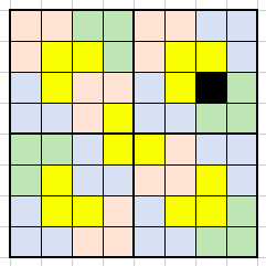
Marking cells: Design an algorithm for the following task. For any even n n n, mark n n n cells on an infinite sheet of graph paper so that each marked cell has an odd number of marked neighbours. Two cells are considered neighbors if they are next to each other either horizontally or vertically but not diagonally. The marked cells must form a contiguous region, i.e., a region in which there is a path between any pair of marked cells that goes through a sequence of marked neighbors. [Kor05]
A: refer to [Algorithmic Puzzles] for detailed solution and analysis.
![[Notes] Introduction to The Design and Analysis of Algorithms from Anany Levitin_第7张图片](http://img.e-com-net.com/image/info8/d959a8da21624b1ca4e305e2ecef7769.png)
4.2 Topological Sorting
Example: consider a set of five required courses {C1, C2, C3, C4, C5} a part-time student has to take in some degree program. The courses can be taken in any order as long as the following course prerequisites are met: C1 and C2 have no prerequisites, C3 requires C1 and C2, C4 requires C3, and C5 requires C3 and C4. The student can take only one course per term. In which order should the student take the courses?
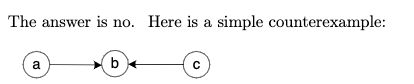
The topological sorting problem has a solution if and only if it is a dag (directed acyclic graph, i.e., no back edges)
Algorithm 1:
The first algorithm is a simple application of depth-first search: perform a DFS traversal and note the order in which vertices become dead-ends (i.e., popped off the traversal stack). Reversing this order yields a solution to the topological sorting problem, provided, of course, no back edge has been encountered during the traversal. If a back edge has been encountered, the digraph is not a dag, and topological sorting of its vertices is impossible.
Q: Why does the algorithm work?
A: When a vertex v v v is popped off a DFS stack, no vertex u u u with an edge from u u u to v v v can be among the vertices popped off before v v v. (Otherwise, ( u , v ) (u, v) (u,v) would have been a back edge.) Hence, any such vertex u u u will be listed after v v v in the popped-off order list, and before v v v in the reversed list.
Algorithm 2:
Based on a direct implementation of the decrease-(by one)-and-conquer technique: repeatedly, identify in a remaining digraph a source, which is a vertex with no incoming edges, and delete it along with all the edges outgoing from it. (If there are several sources, break the tie arbitrarily. If there are none, stop because the problem cannot be solved) The order in which the vertices are deleted yields a solution to the topological sorting problem.
The topological sorting problem may have several alternative solutions.
Q: prove a non-empty dag must have at least one source.
A:
![[Notes] Introduction to The Design and Analysis of Algorithms from Anany Levitin_第8张图片](http://img.e-com-net.com/image/info8/f0ef2917d54a4d70a00d65cc6c7d5441.jpg)
Exercises 4.2
Q: Can one use the order in which vertices are pushed onto the DFS stack (instead of the order they are popped off it) to solve the topological sorting problem?
A:
Topological Sorting from GeeksforGeeks
4.3 Algorithms for Generating Combinatorial Objects
The number of combinatorial objects typically grows exponentially or even faster as a function of the problem size.
Generating Permutations
Decrease-by-one technique: for the problem of generating all n ! n! n! permutations of 1 , . . . , n {1, . . . , n} 1,...,n. The smaller-by-one problem is to generate all ( n − 1 ) ! (n − 1)! (n−1)! permutations. Assuming that the smaller problem is solved, we can get a solution to the larger one by inserting n n n in each of the n n n possible positions among elements of every permutation of n − 1 n − 1 n−1 elements.
We can insert n n n in the previously generated permutations either left to right or right to left. It turns out that it is beneficial to start with inserting n n n into 12... ( n − 1 ) 12 . . . (n − 1) 12...(n−1) by moving right to left and then switch direction every time a new permutation of 1 , . . . , n − 1 {1, . . . , n − 1} 1,...,n−1 needs to be processed.
It satisfies the minimal-change requirement: each permutation can be obtained from its immediate predecessor by exchanging just two elements in it.
Algorithm 1: bottom-up
![[Notes] Introduction to The Design and Analysis of Algorithms from Anany Levitin_第9张图片](http://img.e-com-net.com/image/info8/2c430650db1b4410835256b10609dd27.jpg)
Algorithm 2:
![[Notes] Introduction to The Design and Analysis of Algorithms from Anany Levitin_第10张图片](http://img.e-com-net.com/image/info8/a55e398edcf44d1caf25b70184cba657.jpg)
Algorithm 3:
![[Notes] Introduction to The Design and Analysis of Algorithms from Anany Levitin_第11张图片](http://img.e-com-net.com/image/info8/43811d45af6f4ac08c9ef7c6fafc62ae.jpg)
Algorithm 3: minimum-movement
ALGORITHM HeapPermute(n)
//Implements Heap’s algorithm for generating permutations
//Input: A positive integer n and a global array A[1..n] //Output: All permutations of elements of A
if n = 1
	write A
else
	for i ← 1 to n do
		HeapPermute(n − 1)
		if n is odd
			swap A[1] and A[n]
		else
			swap A[i] and A[n]
Generating Subsets
Implementation 1: squashed order
![[Notes] Introduction to The Design and Analysis of Algorithms from Anany Levitin_第12张图片](http://img.e-com-net.com/image/info8/ff86c02249ef4935bb71ddb8c8c4f7e3.jpg)
Implementation 2: lexicographic order

Implementation 3: binary reflected Gray code
A minimal-change algorithm for generating bit strings so that every one of them differs from its immediate predecessor by only a single bit.
![]()
Recursive version
![[Notes] Introduction to The Design and Analysis of Algorithms from Anany Levitin_第13张图片](http://img.e-com-net.com/image/info8/9c0a71937d8d4f469a9b18bb2571b0a8.jpg)
Non-recursive version
Start with the n n n-bit string of all 0 0 0’s. For i = 1 , 2 , . . . , 2 n − 1 i = 1, 2, . . . , 2n−1 i=1,2,...,2n−1, generate the i t h ith ith bit string by flipping bit b b b in the previous bit string, where b b b is the position of the least significant 1 1 1 in the binary representation of i i i.
Take n=3 as an example:
initialise with 000 000 000
i = 1 → 001 i=1\to001 i=1→001, b = 3 t h b=3th b=3th, 000 → 001 000\to001 000→001
i = 2 → 010 i=2\to010 i=2→010, b = 2 r d b=2rd b=2rd, 001 → 011 001\to011 001→011
i = 3 → 011 i=3\to011 i=3→011, b = 3 t h b=3th b=3th, 011 → 010 011\to010 011→010
i = 4 → 100 i=4\to100 i=4→100, b = 1 s t b=1st b=1st, 010 → 110 010\to110 010→110
i = 5 → 101 i=5\to101 i=5→101, b = 3 t h b=3th b=3th, 110 → 111 110\to111 110→111
i = 6 → 110 i=6\to110 i=6→110, b = 2 r d b=2rd b=2rd, 111 → 101 111\to101 111→101
i = 7 → 111 i=7\to111 i=7→111, b = 3 t h b=3th b=3th, 101 → 100 101\to100 101→100
Exercises 4.3
Q: What simple trick would make the bit string-based algorithm generate subsets in squashed order?
A: Reverse each bit string, for example: 001 -> 100, 010 -> 010, 011 -> 110, etc.
Q: Fair attraction In olden days, one could encounter the following attraction at a fair. A light bulb was connected to several switches in such a way that it lighted up only when all the switches were closed. Each switch was controlled by a push button; pressing the button toggled the switch, but there was no way to know the state of the switch. The object was to turn the light bulb on. Design an algorithm to turn on the light bulb with the minimum number of button pushes needed in the worst case for n switches.
A: Use Gray code non-recursive solution. Because Gray code is cyclic, whatever the state it is for now, it will finally move to all 0 state.
Formula: e = 1 + 1 1 ! + 1 2 ! + ⋯ + 1 n ! e=1+{1\over 1!}+{1\over 2!}+\dots +{1\over n!} e=1+1!1+2!1+⋯+n!1
4.4 Decrease-by-a-Constant-Factor Algorithms
Usually run in logarithmic time.
Binary Search
Search in a sorted array.
It works by comparing a search key K K K with the array’s middle element A [ m ] A[m] A[m]. If they match, the algorithm stops; otherwise, the same operation is repeated recursively for the first half of the array if K < A [ m ] K < A[m] K<A[m], and for the second half if K > A [ m ] K > A[m] K>A[m].
![[Notes] Introduction to The Design and Analysis of Algorithms from Anany Levitin_第14张图片](http://img.e-com-net.com/image/info8/c7705b0a4b8f49f093f656364badc548.jpg)
The basic operation is the comparison between the search key and an element of the array. We consider three-way comparisons here.
C w o r s t ( n ) = C w o r s t ( ⌊ n / 2 ⌋ ) + 1 f o r n > 1 , C w o r s t ( 1 ) = 1 C_{worst}(n)=C_{worst}(\lfloor n/2 \rfloor)+1\space for\space n>1,C_{worst}(1)=1 Cworst(n)=Cworst(⌊n/2⌋)+1 for n>1,Cworst(1)=1 C w o r s t ( n ) = ⌊ log 2 n ⌋ ) + 1 = ⌈ log 2 n + 1 ⌉ ∈ Θ ( log n ) C_{worst}(n)=\lfloor\log_2{n}\rfloor)+1=\lceil\log_2{n+1}\rceil\in\Theta(\log n) Cworst(n)=⌊log2n⌋)+1=⌈log2n+1⌉∈Θ(logn)The average number of key comparisons made by binary search is only slightly smaller than that in the worst case: C a v g ( n ) ≈ log 2 n C_{avg}(n)\approx\log_2 n Cavg(n)≈log2n C a v g y e s ( n ) ≈ log 2 n − 1 C_{avg}^{yes}(n)\approx\log_2 n-1 Cavgyes(n)≈log2n−1 C a v g n o ( n ) ≈ log 2 ( n + 1 ) C_{avg}^{no}(n)\approx\log_2(n+1) Cavgno(n)≈log2(n+1)
Josephus Problem
J ( 2 k ) = 2 J ( k ) − 1 J(2k) = 2J(k) − 1 J(2k)=2J(k)−1 J ( 2 k + 1 ) = 2 J ( k ) + 1 J (2k + 1) = 2J (k) + 1 J(2k+1)=2J(k)+1The most elegant form of the closed-form answer involves the binary representation of size n n n: J ( n ) J (n) J(n) can be obtained by a 1-bit cyclic shift left of n n n itself: J ( 6 ) = J ( 11 0 2 ) = 10 1 2 = 5 , J ( 7 ) = J ( 11 1 2 ) = 11 1 2 = 7 J(6) = J(110_2) = 101_2 = 5,J(7) = J(111_2) = 111_2 = 7 J(6)=J(1102)=1012=5,J(7)=J(1112)=1112=7.
Exercises 4.4
Q: Cutting a Stick A stick 100 100 100 units long needs to be cut into 100 100 100 unit pieces. What is the minimum number of cuts required if you are allowed to cut several stick pieces at the same time? Also outline an algorithm that performs this task with the minimum number of cuts for a stick of n n n units long.
A:
![[Notes] Introduction to The Design and Analysis of Algorithms from Anany Levitin_第15张图片](http://img.e-com-net.com/image/info8/5acc532d277d4e48802f86841efaaa89.jpg)
![[Notes] Introduction to The Design and Analysis of Algorithms from Anany Levitin_第16张图片](http://img.e-com-net.com/image/info8/8a95a5a5aac5439191e1265cc6170597.jpg)
![[Notes] Introduction to The Design and Analysis of Algorithms from Anany Levitin_第17张图片](http://img.e-com-net.com/image/info8/4cd6f14468f44c348888a940e4bb5554.jpg)
Q: An array A [ 0.. n − 2 ] A[0..n − 2] A[0..n−2] contains n − 1 n − 1 n−1 integers from 1 1 1 to n n n in increasing order. (Thus one integer in this range is missing.) Design the most efficient algorithm you can to find the missing integer and indicate its time efficiency.
A:
![[Notes] Introduction to The Design and Analysis of Algorithms from Anany Levitin_第18张图片](http://img.e-com-net.com/image/info8/dfcf32bd69d140979c896b1f50f96396.jpg)
Find the Missing Number in a sorted array
Find the Missing Number
4.5 Variable-Size-Decrease Algorithms
Computing a Median and the Selection Problem
The selection problem is the problem of finding the k t h kth kth smallest element in a list of n n n numbers. This number is called the k t h kth kth order statistic.
A more interesting case of this problem is for k = ⌈ n / 2 ⌉ k=\lceil n/2\rceil k=⌈n/2⌉, which asks to find an element that is not larger than one half of the list’s elements and not smaller than the other half which is the median.
Partitioning idea can give us an efficient solution instead of sorting the entire list and finding the k t h kth kth element in the non-decreasing list whose efficiency is determined by the sorting algorithm.
This is a rearrangement of the list’s elements so that the left part contains all the elements smaller than or equal to p p p, followed by the pivot p p p itself, followed by all the elements greater than or equal to p p p.
![[Notes] Introduction to The Design and Analysis of Algorithms from Anany Levitin_第19张图片](http://img.e-com-net.com/image/info8/d9b3e6e067fd4a92a29ac927161a2058.jpg)
Quickselect
Recursive version
Assume that the list is implemented as an array whose elements are indexed starting with a 0 0 0, and s s s is the partition’s split position.
If s = k − 1 s = k − 1 s=k−1, pivot p p p itself is obviously the k t h kth kth smallest element, which solves the problem.
If s > k − 1 s > k − 1 s>k−1, the k t h kth kth smallest element in the entire array can be found as the k t h kth kth smallest element in the left part of the partitioned array.
If s < k − 1 s < k − 1 s<k−1, it can be found as the ( k − s − 1 ) t h (k-s-1)th (k−s−1)th smallest element in its right part.
![[Notes] Introduction to The Design and Analysis of Algorithms from Anany Levitin_第20张图片](http://img.e-com-net.com/image/info8/809862985e2745b3bf699c34938e5ec1.jpg)
*Should be if s=l+k-1 return A[s] ![[Notes] Introduction to The Design and Analysis of Algorithms from Anany Levitin_第21张图片](http://img.e-com-net.com/image/info8/3928cf4e705449ad81528acd83384b44.jpg) Non-recursive version
Non-recursive version
The same idea can be implemented without recursion as well. For the non-recursive version, there is no need to adjust the value of k k k but continue until s = k − 1 s = k − 1 s=k−1.
Interpolation Search
Search in a sorted array.
This algorithm assumes that the array values increase linearly, i.e., along the straight line through the points ( l , A [ l ] ) (l, A[l]) (l,A[l]) and ( r , A [ r ] ) (r, A[r]) (r,A[r]).
The accuracy of this assumption can influence the algorithm’s efficiency but not its correctness. x = l + ⌊ ( v − A [ l ] ) ( r − l ) A [ r ] − A [ l ] ⌋ x=l+\lfloor{{(v-A[l])(r-l)}\over{A[r]-A[l]}}\rfloor x=l+⌊A[r]−A[l](v−A[l])(r−l)⌋
After comparing v v v with A [ x ] A[x] A[x], the algorithm stops if they are equal or proceeds by searching in the same manner among the elements indexed either between l l l and x − 1 x − 1 x−1 or between x + 1 x + 1 x+1 and r r r, depending on whether A [ x ] A[x] A[x] is smaller or larger than v v v. Thus, the size of the problem’s instance is reduced, but we cannot tell a priori by how much.
![[Notes] Introduction to The Design and Analysis of Algorithms from Anany Levitin_第22张图片](http://img.e-com-net.com/image/info8/f4ae67d9219c4fc3a5b5bbf183bfa16d.png)
Searching and Insertion in a Binary Search Tree
In the worst case of the binary tree search, the tree is severely skewed. This happens, in particular, if a tree is constructed by successive insertions of an increasing or decreasing sequence of keys.
![[Notes] Introduction to The Design and Analysis of Algorithms from Anany Levitin_第23张图片](http://img.e-com-net.com/image/info8/eea167b2282646d58264cd481525e748.jpg)
The Game of Nim
One-pile Nim: refer to the explanation in the book.
General solution: very interesting!
![[Notes] Introduction to The Design and Analysis of Algorithms from Anany Levitin_第24张图片](http://img.e-com-net.com/image/info8/41f177a72b504fdc927ee7579efa8c7b.jpg)
![[Notes] Introduction to The Design and Analysis of Algorithms from Anany Levitin_第25张图片](http://img.e-com-net.com/image/info8/a54146cd1abe437ebfc04ce9e853aa9a.jpg)
5. Divide-and-Conquer
- A problem is divided into several subproblems of the same type, ideally of about equal size.
- The subproblems are solved (typically recursively, though sometimes a different algorithm is employed, especially when subproblems become small enough).
- If necessary, the solutions to the subproblems are combined to get a solution to the original problem.
Actually, the divide-and-conquer algorithm, called the pairwise summation, may substantially reduce the accumulated round-off error of the sum of numbers that can be represented only approximately in a digital computer [Hig93].
The divide-and-conquer technique is ideally suited for parallel computations, in which each subproblem can be solved simultaneously by its own processor.
More generally, an instance of size n n n can be divided into b b b instances of size n / b n/b n/b, with a a a of them needing to be solved. (Here, a a a and b b b are constants; a ≥ 1 a ≥ 1 a≥1 and b > 1 b > 1 b>1.) Assuming that size n n n is a power of b b b to simplify our analysis, we get the following recurrence for the running time T ( n ) T (n) T(n): T ( n ) = a T ( n / b ) + f ( n ) T(n)=aT(n/b)+f(n) T(n)=aT(n/b)+f(n)
where f ( n ) f (n) f(n) is a function that accounts for the time spent on dividing an instance of size n n n into instances of size n / b n/b n/b and combining their solutions.
![[Notes] Introduction to The Design and Analysis of Algorithms from Anany Levitin_第26张图片](http://img.e-com-net.com/image/info8/c9930f06d6b24ccb8e2388a3c6c3bdac.jpg)
5.1 Mergesort
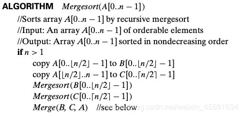
![[Notes] Introduction to The Design and Analysis of Algorithms from Anany Levitin_第27张图片](http://img.e-com-net.com/image/info8/145cd2af38a4488ba6e87ffc517ac656.jpg)
Explanation:
The merging of two sorted arrays can be done as follows. Two pointers (array indices) are initialized to point to the first elements of the arrays being merged. The elements pointed to are compared, and the smaller of them is added to a new array being constructed; after that, the index of the smaller element is incremented to point to its immediate successor in the array it was copied from. This operation is repeated until one of the two given arrays is exhausted, and then the remaining elements of the other array are copied to the end of the new array.
Effciency:
C ( n ) = 2 C ( n / 2 ) + C m e r g e ( n ) f o r n > 1 , C ( 1 ) = 0. C(n) = 2C(n/2) + C_{merge}(n) for\space n > 1, C(1) = 0. C(n)=2C(n/2)+Cmerge(n)for n>1,C(1)=0.
C w o r s t ( n ) = 2 C w o r s t ( n / 2 ) + n − 1 f o r n > 1 , C w o r s t ( 1 ) = 0. C_{worst}(n) = 2C_{worst}(n/2) + n − 1\space for\space n > 1, C_{worst}(1) = 0. Cworst(n)=2Cworst(n/2)+n−1 for n>1,Cworst(1)=0.
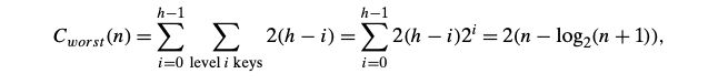
Exact solution to the worst-case recurrence for n = 2 k : C w o r s t ( n ) = n l o g 2 n − n + 1. n = 2^k: C_{worst}(n)=nlog_{2}n−n+1. n=2k:Cworst(n)=nlog2n−n+1.
Advantages:
-
The number of key comparisons made by mergesort in the worst case comes very close to the theoretical minimum ⌈ l o g 2 n ! ⌉ ≈ ⌈ n l o g 2 n − 1.44 n ⌉ ⌈log_2 n!⌉ ≈ ⌈n log_2 n − 1.44n⌉ ⌈log2n!⌉≈⌈nlog2n−1.44n⌉ that any general comparison-based sorting algorithm can have. For large n n n, the number of comparisons made by this algorithm in the average case turns out to be about 0.25 n 0.25n 0.25n less (see [Gon91, p. 173]) and hence is also in Θ ( n l o g n ) \Theta(n log n) Θ(nlogn).
-
A noteworthy advantage of mergesort over quicksort and heapsort—the two important advanced sorting algorithms to be discussed later—is its stability.
Shortcomings
- The algorithm requires linear amount of extra storage.
- Though merging can be done in-place, the resulting algorithm is quite complicated and of theoretical interest only.
Improvements:
- The algorithm can be implemented bottom up by merging pairs of the array’s elements, then merging the sorted pairs, and so on.
- Multiway mergesort: divide a list to be sorted in more than two parts, sort each recursively, and then merge them together.
Exercises 5.1
Problem 11:
5.2 Quicksort
The difference with mergesort: the entire work happens in the division stage, with no work required to combine the solutions to the subproblems (with no need to merge two subarrays into one).
![[Notes] Introduction to The Design and Analysis of Algorithms from Anany Levitin_第28张图片](http://img.e-com-net.com/image/info8/7b1bfc362281471393e8c943e475afe1.jpg)
![[Notes] Introduction to The Design and Analysis of Algorithms from Anany Levitin_第29张图片](http://img.e-com-net.com/image/info8/bb484b2ecd7540be90eb376cbba3bcd3.jpg)
Index i i i can go out of the subarray’s bounds in the above pseudocode, we can append a “sentinel” that would prevent index i i i from advancing beyond position n n n to the end of the array.
Efficiency analysis:
1. Best case:
The number of key comparisons made before a partition is achieved is n + 1 n + 1 n+1 if the scanning indices cross over and n n n if they coincide. If all the splits happen in the middle of corresponding subarrays, we will have the best case. The number of key comparisons in the best case satisfies the recurrence:
C b e s t ( n ) = 2 C b e s t ( n / 2 ) + n f o r n > 1 , C b e s t ( 1 ) = 0. C_{best}(n) = 2C_{best}(n/2) + n\space for\space n > 1, C_{best}(1) = 0. Cbest(n)=2Cbest(n/2)+n for n>1,Cbest(1)=0. C b e s t ( n ) ∈ Θ ( n l o g 2 n ) C_{best}(n) ∈ \Theta(n log_2 n) Cbest(n)∈Θ(nlog2n) C b e s t ( n ) = n l o g 2 n f o r n = 2 k . C_{best}(n) = nlog_2n\space\space for\space\space n = 2k. Cbest(n)=nlog2n for n=2k.
2. Worst case:
The worst case is when A [ 0.. n − 1 ] A[0..n − 1] A[0..n−1] is a strictly increasing array, the total number of key comparisons made will be equal to:
![]()
3. Average case:
A partition can happen in any position s ( 0 ≤ s ≤ n − 1 ) s (0 ≤ s ≤ n − 1) s(0≤s≤n−1) after n + 1 n + 1 n+1 comparisons are made to achieve the partition. After the partition, the left and right subarrays will have s s s and n − 1 − s n − 1 − s n−1−s elements, respectively. Assuming that the partition split can happen in each position s s s with the same probability 1 / n 1/n 1/n, we get the following recurrence relation:

![]()
On the average, quicksort makes only 39% more comparisons than in the best case. Moreover, its innermost loop is so efficient that it usually runs faster than mergesort and heapsort on randomly ordered arrays of non-trivial sizes.
Improvements:
![[Notes] Introduction to The Design and Analysis of Algorithms from Anany Levitin_第30张图片](http://img.e-com-net.com/image/info8/7b1185b0a8684614a22e2c93e4b3e11a.jpg)
Weaknesses: not stable.
5.3 Binary Tree Traversals and Related Properties
The height is defined as the length of the longest path from the root to a leaf. => the maximum of the heights of the root’s left and right subtrees plus 1. (We have to add 1 to account for the extra level of the root.)
Also note that it is convenient to define the height of the empty tree as −1.
![[Notes] Introduction to The Design and Analysis of Algorithms from Anany Levitin_第31张图片](http://img.e-com-net.com/image/info8/a8a219b0632246b4a34657de07cf27b0.jpg)
Efficiency analysis:

Checking that the tree is not empty is the most frequently executed operation of this algorithm and this is very typical for binary tree algorithms.
Trick: Replace the empty subtrees by special nodes called external which is different from original nodes called internal.
Height algorithm makes exactly one addition for every internal node of the extended tree, and it makes one comparison to check whether the tree is empty for every internal and external node.
The number of additions is A ( n ) = n A(n) = n A(n)=n, comparison is A ( n ) = 2 n + 1 A(n) = 2n + 1 A(n)=2n+1.
5.4 Multiplication of Large Integers and Strassen’s Matrix Multiplication
Multiplication of Large Integers
![[Notes] Introduction to The Design and Analysis of Algorithms from Anany Levitin_第32张图片](http://img.e-com-net.com/image/info8/f329af798bb74e06a71da1711ae24943.jpg)
![[Notes] Introduction to The Design and Analysis of Algorithms from Anany Levitin_第33张图片](http://img.e-com-net.com/image/info8/c364095af8274af1887b6f37b20a984f.jpg)
![[Notes] Introduction to The Design and Analysis of Algorithms from Anany Levitin_第34张图片](http://img.e-com-net.com/image/info8/aff36b997ab6457e9da0f4bf688e8158.jpg)
If additions and subtractions are included in the analysis of efficiency: A ( n ) = 3 A ( n / 2 ) + c n f o r n > 1 , A ( 1 ) = 1. A(n)=3A(n/2)+cn\space for\space n>1, A(1)=1. A(n)=3A(n/2)+cn for n>1,A(1)=1.
Applying the Master Theorem, A ( n ) ∈ Θ ( n l o g 2 3 ) A(n) ∈ \Theta(n^{log_23}) A(n)∈Θ(nlog23)
Strassen’s Matrix Multiplication
![[Notes] Introduction to The Design and Analysis of Algorithms from Anany Levitin_第35张图片](http://img.e-com-net.com/image/info8/561606f9189d4df58ce6cca420bc122d.jpg)
![[Notes] Introduction to The Design and Analysis of Algorithms from Anany Levitin_第36张图片](http://img.e-com-net.com/image/info8/5df957fafee64ef4b523e6afbfad9f09.jpg)
![[Notes] Introduction to The Design and Analysis of Algorithms from Anany Levitin_第37张图片](http://img.e-com-net.com/image/info8/5bffda0680544669b746ca300ae7f930.jpg)
If only multiplication is included in the analysis:
![[Notes] Introduction to The Design and Analysis of Algorithms from Anany Levitin_第38张图片](http://img.e-com-net.com/image/info8/55963a67cac84e9c8eb3d49c80348f22.jpg)
To multiply two matrices of order n > 1 n > 1 n>1, the algorithm needs to multiply seven matrices of order n / 2 n/2 n/2 and make 18 18 18 additions/subtractions of matrices of size n / 2 n/2 n/2 ; when n = 1 n = 1 n=1, no additions are made. A ( n ) = 7 A ( n / 2 ) + 18 ( n / 2 ) 2 f o r n > 1 , A ( 1 ) = 0. A(n)=7A(n/2)+18(n/2)^2 \space for\space n>1, A(1)=0. A(n)=7A(n/2)+18(n/2)2 for n>1,A(1)=0.
According to the Master Theorem, A ( n ) ∈ Θ ( n l o g 2 7 ) . A(n) ∈ \Theta(n^{log_27}). A(n)∈Θ(nlog27).
5.5 The Closest-Pair and Convex-Hull Problems by Divide-and-Conquer
The Closest-Pair Problem
![[Notes] Introduction to The Design and Analysis of Algorithms from Anany Levitin_第39张图片](http://img.e-com-net.com/image/info8/8dc0027db32045aeb4ac8da130f39299.jpg)
![[Notes] Introduction to The Design and Analysis of Algorithms from Anany Levitin_第40张图片](http://img.e-com-net.com/image/info8/781d9696640c4856a5f09d60a0e4650b.jpg)
Convex-Hull Problem
See the book.
6. Transform-and-Conquer
Instance simplification: Transformation to a simpler or more convenient instance of the same problem.
Representation change: Transformation to a different representation of the same instance.
Problem reduction: Transformation to an instance of a different problem for which an algorithm is already available.
6.1 Presorting
Three elementary sorting algorithms—selection sort, bubble sort, and insertion sort—that are quadratic in the worst and average cases, and two advanced algorithms—mergesort, which is always in Θ ( n l o g n ) \Theta(nlogn) Θ(nlogn), and quicksort, whose efficiency is also Θ ( n l o g n ) \Theta(nlogn) Θ(nlogn)) in the average case but is quadratic in the worst case.
No general comparison-based sorting algorithm can have a better efficiency than n l o g n n log n nlogn in the worst case, and the same result holds for the average-case efficiency.
![[Notes] Introduction to The Design and Analysis of Algorithms from Anany Levitin_第41张图片](http://img.e-com-net.com/image/info8/ca87bb4347914eb5a1cdcc180031fb44.jpg)
Sorting part that will determine the overall efficiency of the algorithm. If a good sorting algorithm is used, such as mergesort, with worst-case efficiency in Θ ( n l o g n ) \Theta(n log n) Θ(nlogn), the worst-case efficiency of the entire presorting-based algorithm will be also in Θ ( n l o g n ) \Theta(n log n) Θ(nlogn): T ( n ) = T s o r t ( n ) + T s c a n ( n ) ∈ Θ ( n l o g n ) + Θ ( n ) = Θ ( n l o g n ) T (n) = T_{sort}(n) + T_{scan}(n) ∈ \Theta(n log n) + \Theta(n) = \Theta(n log n) T(n)=Tsort(n)+Tscan(n)∈Θ(nlogn)+Θ(n)=Θ(nlogn)![]()
![[Notes] Introduction to The Design and Analysis of Algorithms from Anany Levitin_第42张图片](http://img.e-com-net.com/image/info8/d32ac41e0f554e69a0e46a6dbe258341.jpg)
The running time of the algorithm will be dominated by the time spent on sorting since the remainder of the algorithm takes linear time.
![[Notes] Introduction to The Design and Analysis of Algorithms from Anany Levitin_第43张图片](http://img.e-com-net.com/image/info8/114b1ab41a1844f2ad1439996a4fc95d.jpg)
![[Notes] Introduction to The Design and Analysis of Algorithms from Anany Levitin_第44张图片](http://img.e-com-net.com/image/info8/4835fa227fef416eac5451b033eb00c8.jpg)
Exercises 6.1
![[Notes] Introduction to The Design and Analysis of Algorithms from Anany Levitin_第45张图片](http://img.e-com-net.com/image/info8/dcd334ba496c4f4888712c8e7fe03732.jpg)
Solution reference
The from looking at the question we can say the numbers be sorted and if less than symbol appears next we have to insert the least number, if greater than symbol appears we have to insert max number and proceed as so.
#Python code
def less(syms, i, j):
    if i == j: return False
    s = '<' if i < j else '>'
    return all(c == s for c in syms[min(i,j):max(i,j)])

def order(boxes, syms):
    if not boxes:
        yield []
        return
    for x in [b for b in boxes if not any(less(syms, a, b) for a in boxes)]:
        for y in order(boxes - set([x]), syms):
            yield [x] + y

def solutions(syms):
    for idxes in order(set(range(len(syms)+1)), syms):
        yield [idxes.index(i) for i in range(len(syms)+1)]

print(list(solutions('<><<')))
All possible solutions:

[[0, 2, 1, 3, 4],
[0, 3, 1, 2, 4],
[0, 4, 1, 2, 3],
[1, 2, 0, 3, 4],
[1, 3, 0, 2, 4],
[1, 4, 0, 2, 3],
[2, 3, 0, 1, 4],
[2, 4, 0, 1, 3],
[3, 4, 0, 1, 2]]
![[Notes] Introduction to The Design and Analysis of Algorithms from Anany Levitin_第46张图片](http://img.e-com-net.com/image/info8/66e55475f4d14d36b1ee3b0e653488cb.jpg)
LightsOutPuzzle
6.2 Guassian Elimination
![[Notes] Introduction to The Design and Analysis of Algorithms from Anany Levitin_第47张图片](http://img.e-com-net.com/image/info8/d5010ec82475483d83c23fb311b764cc.jpg)
Elementary operations to get an equivalent system with an upper-triangular coefficient matrix A:
- exchanging two equations of the system
- replacing an equation with its nonzero multiple
- replacing an equation with a sum or difference of this equation and some multiple of another equation
![[Notes] Introduction to The Design and Analysis of Algorithms from Anany Levitin_第48张图片](http://img.e-com-net.com/image/info8/7df7e3c0af824495a3862aa64a981a33.jpg)
Improvement:
-
First, it is not always correct: if A [ i , i ] = 0 A[i, i] = 0 A[i,i]=0, we cannot divide by it and hence cannot use the i t h ith ith row as a pivot for the i t h ith ith iteration of the algorithm
==> we should exchange the i t h ith ith row with some row below it that has a nonzero coefficient in the i t h ith ith column. (If the system has a unique solution, which is the normal case for systems under consideration, such a row must exist.)
-
he possibility that A [ i , i ] A[i, i] A[i,i] is so small and consequently the scaling factor A [ j , i ] / A [ i , i ] A[j, i]/A[i, i] A[j,i]/A[i,i] so large that the new value of A [ j , k ] A[j, k] A[j,k] might become distorted by a round-off error caused by a subtraction of two numbers of greatly different magnitude
==> Partial pivoting: always look for a row with the largest absolute value of the coefficient in the i t h ith ith column, exchange it with the i t h ith ith row, and then use the new A [ i , i ] A[i, i] A[i,i] as the i t h ith ith iteration’s pivot. (guarantee the magnitude of scaling factor will never exceed 1)
![[Notes] Introduction to The Design and Analysis of Algorithms from Anany Levitin_第49张图片](http://img.e-com-net.com/image/info8/46b2a0a486fb42c9b79a9cca27b6d3af.jpg)
![[Notes] Introduction to The Design and Analysis of Algorithms from Anany Levitin_第50张图片](http://img.e-com-net.com/image/info8/14c39adf6688461f8ceb21c886b389fc.jpg)
Applications:
- LU Decomposition
- Computing a Matrix Inverse
- Computing a Determinant
6.3 Balanced Search Trees
![[Notes] Introduction to The Design and Analysis of Algorithms from Anany Levitin_第51张图片](http://img.e-com-net.com/image/info8/e31e6d3840b24a1798e007c0ca601812.jpg)
![[Notes] Introduction to The Design and Analysis of Algorithms from Anany Levitin_第52张图片](http://img.e-com-net.com/image/info8/f8932128c1844757811f803cc3da366a.jpg)
![[Notes] Introduction to The Design and Analysis of Algorithms from Anany Levitin_第53张图片](http://img.e-com-net.com/image/info8/e484a352b7824b62a3670b838aee390d.png)
AVL tree
![[Notes] Introduction to The Design and Analysis of Algorithms from Anany Levitin_第54张图片](http://img.e-com-net.com/image/info8/9e52bd9a478a4c40963a0f5fe1ca41cb.png)

Single right rotation, or R-rotation: rotate the edge connecting the root and its left child in the binary tree to the right.
![[Notes] Introduction to The Design and Analysis of Algorithms from Anany Levitin_第55张图片](http://img.e-com-net.com/image/info8/2eb0f79ba616438bbc31d648d422131a.jpg)
Single left rotation, or L-rotation:
![[Notes] Introduction to The Design and Analysis of Algorithms from Anany Levitin_第56张图片](http://img.e-com-net.com/image/info8/61282173be94492e999688bc26df6946.jpg)
Double left-right rotation (LR- rotation): perform the L-rotation of the left subtree of root r followed by the R-rotation of the new tree rooted at r.
![[Notes] Introduction to The Design and Analysis of Algorithms from Anany Levitin_第57张图片](http://img.e-com-net.com/image/info8/aa6781b7b2584110b8c4236c24a9322a.jpg)
Double right-left rotation (RL-rotation)
![[Notes] Introduction to The Design and Analysis of Algorithms from Anany Levitin_第58张图片](http://img.e-com-net.com/image/info8/e411347f3669455096938f1a5595b91c.jpg)
Keep in mind that if there are several nodes with the ±2 balance, the rotation is done for the tree rooted at the unbalanced node that is the closest to the newly inserted leaf.
![[Notes] Introduction to The Design and Analysis of Algorithms from Anany Levitin_第59张图片](http://img.e-com-net.com/image/info8/bc24b0ad629543329ac89cf640df7bc1.jpg)
Efficiency analysis:
Height h h h of any AVL tree with n n n nodes satisfies the inequalities ⌊ l o g 2 n ⌋ ≤ h < 1.4405 l o g 2 ( n + 2 ) − 1.3277 ⌊log2 n⌋ ≤ h < 1.4405 log_2(n + 2) − 1.3277 ⌊log2n⌋≤h<1.4405log2(n+2)−1.3277
![[Notes] Introduction to The Design and Analysis of Algorithms from Anany Levitin_第60张图片](http://img.e-com-net.com/image/info8/6a3d1da4f4c0479bbae0f365c0e1b8d9.jpg)

2-3 Trees
![[Notes] Introduction to The Design and Analysis of Algorithms from Anany Levitin_第61张图片](http://img.e-com-net.com/image/info8/5745cef267f7474c96d25bc62831c8f6.jpg)
All its leaves must be on the same level. In other words, a 2-3 tree is always perfectly height-balanced: the length of a path from the root to a leaf is the same for every leaf.
![[Notes] Introduction to The Design and Analysis of Algorithms from Anany Levitin_第62张图片](http://img.e-com-net.com/image/info8/2e9fbacbf82548ca95b3865e857255cb.jpg)
![[Notes] Introduction to The Design and Analysis of Algorithms from Anany Levitin_第63张图片](http://img.e-com-net.com/image/info8/d57539db6b794495bed5e87e441f1f78.jpg)
Efficiency analysis:
l o g 3 ( n + 1 ) − 1 ≤ h ≤ l o g 2 ( n + 1 ) − 1 log_3(n+1)−1≤h≤log_2(n+1)−1 log3(n+1)−1≤h≤log2(n+1)−1
imply that the time efficiencies of searching, insertion, and deletion are all in Θ ( l o g n ) \Theta(log n) Θ(logn) in both the worst and average case.
6.4 Heaps and Heapsort
Heap is a clever, partially ordered data structure that is especially suitable for implementing priority queues.
Operations:
- finding an item with the highest (i.e., largest) priority
- deleting an item with the highest priority
- adding a new item to the multiset
![[Notes] Introduction to The Design and Analysis of Algorithms from Anany Levitin_第64张图片](http://img.e-com-net.com/image/info8/d34184ce172442c08be66fd7795a9917.jpg)
Key values in a heap are ordered top down; i.e., a sequence of values on any path from the root to a leaf is decreasing (non-increasing, if equal keys are allowed).
Properties:
![[Notes] Introduction to The Design and Analysis of Algorithms from Anany Levitin_第65张图片](http://img.e-com-net.com/image/info8/0094fa5c9fd241a7a6d6508ef56fc7b0.jpg)
Bottom-up heap construction
![[Notes] Introduction to The Design and Analysis of Algorithms from Anany Levitin_第66张图片](http://img.e-com-net.com/image/info8/a2240046c0eb4f50a64027be95d2dca2.jpg)
Top-down heap construction
![[Notes] Introduction to The Design and Analysis of Algorithms from Anany Levitin_第67张图片](http://img.e-com-net.com/image/info8/7101218385fc4cf993128ac6415dfa36.png)
This insertion operation cannot require more key comparisons than the heap’s height. Since the height of a heap with n n n nodes is about l o g 2 n log_2n log2n, the time efficiency of insertion is in O ( l o g n ) O(log n) O(logn).
Deleting the root’s key from a heap:
![[Notes] Introduction to The Design and Analysis of Algorithms from Anany Levitin_第68张图片](http://img.e-com-net.com/image/info8/a709121b9f224f2e9274198320c2f727.jpg)
The time efficiency of deletion is in O ( l o g n ) O(log n) O(logn) as well.
Heapsort

![[Notes] Introduction to The Design and Analysis of Algorithms from Anany Levitin_第69张图片](http://img.e-com-net.com/image/info8/0d05e09030554d3d9d6a51419754ac99.jpg)
6.5 Horner’s Rule and Binary Exponentiation
Horner’s Rule
The problem of computing the value of a polynomial at a given point x is important for fast Fourier transform (FFT) algorithm.
![]()
![[Notes] Introduction to The Design and Analysis of Algorithms from Anany Levitin_第70张图片](http://img.e-com-net.com/image/info8/532f57bae4ad413d92d21c2296f5034b.jpg)
Except for its first entry, which is a n a_n an, the second row is filled left to right as follows: the next entry is computed as the x x x’s value times the last entry in the second row plus the next coefficient from the first row. The final entry computed in this fashion is the value being sought.
![[Notes] Introduction to The Design and Analysis of Algorithms from Anany Levitin_第71张图片](http://img.e-com-net.com/image/info8/9ff000ad16394a91b66925a348e2edac.jpg)
![[Notes] Introduction to The Design and Analysis of Algorithms from Anany Levitin_第72张图片](http://img.e-com-net.com/image/info8/b2add107ec4d4e8d9502c988583c94b8.jpg)
Efficiency analysis:
![[Notes] Introduction to The Design and Analysis of Algorithms from Anany Levitin_第73张图片](http://img.e-com-net.com/image/info8/72c493e9bb854ce896c4817aa788d184.jpg)
Just computing this single term by the brute-force algorithm would require n n n multiplications, whereas Horner’s rule computes, in addition to this term, n − 1 n − 1 n−1 other terms, and it still uses the same number of multiplications!
Synthetic division: Horner’s rule also has some useful byproducts. The intermediate numbers generated by the algorithm in the process of evaluating p ( x ) p(x) p(x) at some point x 0 x_0 x0 turn out to be the coefficients of the quotient of the division of p ( x ) p(x) p(x) by x − x 0 x − x_0 x−x0, and the final result, in addition to being p ( x 0 ) p(x_0) p(x0), is equal to the remainder of this division. 2 x 4 − x 3 + 3 x 2 + x − 5 = ( x − 3 ) ∗ ( 2 x 3 + 5 x 2 + 18 x + 55 ) + 160 2x^4 − x^3 + 3x^2 + x − 5 = (x − 3) * (2x^3 + 5x^2 + 18x + 55) + 160 2x4−x3+3x2+x−5=(x−3)∗(2x3+5x2+18x+55)+160 W h e n x = 3 , 2 x 4 − x 3 + 3 x 2 + x − 5 = 160 When\space x = 3, 2x^4 − x^3 + 3x^2 + x − 5 = 160 When x=3,2x4−x3+3x2+x−5=160
Binary Exponentiation
![[Notes] Introduction to The Design and Analysis of Algorithms from Anany Levitin_第74张图片](http://img.e-com-net.com/image/info8/7037e9ffd337419dac431c4feff5d97a.jpg)
![[Notes] Introduction to The Design and Analysis of Algorithms from Anany Levitin_第75张图片](http://img.e-com-net.com/image/info8/730eb9f7344d46989f37abc71aae2e3c.jpg)
Thus, after initializing the accumulator’s value to a a a, we can scan the bit string representing the exponent n n n to always square the last value of the accumulator and, if the current binary digit is 1, also to multiply it by a a a. These observations lead to the following left-to-right binary exponentiation method of computing a n a^n an.
![[Notes] Introduction to The Design and Analysis of Algorithms from Anany Levitin_第76张图片](http://img.e-com-net.com/image/info8/d6f016cbca8f4a52bd516ec99617d64f.jpg)
Efficiency analysis:
b b b is the length of the bit string representing the exponent n n n:
( b − 1 ) ≤ M ( n ) ≤ 2 ( b − 1 ) , M : m u l t i p l i c a t i o n s (b − 1) ≤ M(n) ≤ 2(b − 1), M: multiplications (b−1)≤M(n)≤2(b−1),M:multiplications b − 1 = ⌊ l o g 2 n ⌋ b − 1 = ⌊log2 n⌋ b−1=⌊log2n⌋
This algorithm is in a logarithm efficiency class, which is better than the brute-force exponentiation, which always requires n − 1 n − 1 n−1 multiplications.
![[Notes] Introduction to The Design and Analysis of Algorithms from Anany Levitin_第77张图片](http://img.e-com-net.com/image/info8/d8cf968b4ed74839b11eff39485cd421.jpg)
![[Notes] Introduction to The Design and Analysis of Algorithms from Anany Levitin_第78张图片](http://img.e-com-net.com/image/info8/3907a82c62184a999f8edbdc330036c9.jpg)
Similar efficiency as the LeftRightBinaryExponentiation. But, the usefulness of both binary exponentiation algorithms is reduced somewhat by their reliance on availability of the explicit binary expansion of exponent n n n.
6.6 Problem Reduction
The practical difficulty in applying it lies, of course, in finding a problem to which the problem at hand should be reduced.
In fact, the entire idea of analytical geometry is based on reducing geometric problems to algebraic ones.
Computing the Least Common Multiple
Drawbacks for middle-school algorithm: inefficient and requires a list of consecutive primes (same as middle-school algorithm forn computing the greatest common divisor)
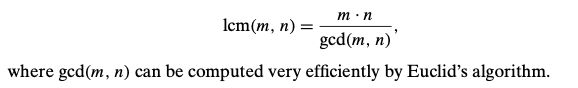
Counting Paths in a Graph
The number of different paths of length k > 0 k > 0 k>0 from the i t h ith ith vertex to the j t h jth jth vertex of a graph (undirected or directed) equals the ( i , j ) t h (i, j )th (i,j)th element of A k A_k Ak where A A A is the adjacency matrix of the graph.
Therefore, the problem of counting a graph’s paths can be solved with an algorithm for computing an appropriate power of its adjacency matrix.
Reduction of Optimization Problems
m i n f ( x ) = − m a x [ − f ( x ) ] . min f (x) = − max[−f (x)]. minf(x)=−max[−f(x)]. m a x f ( x ) = − m i n [ − f ( x ) ] max f (x) = − min[−f (x)] maxf(x)=−min[−f(x)]
Linear Programming
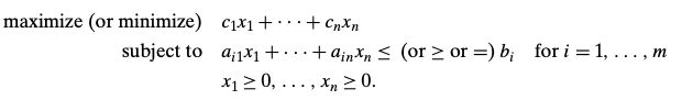
The classic algorithm for this problem is called the simplex method. Although the worst-case efficiency of this algorithm is known to be exponential, it performs very well on typical inputs. Moreover, a more recent algorithm by Narendra Karmarkar [Kar84] not only has a proven polynomial worst-case efficiency but has also performed competitively with the simplex method in empirical tests.
Integer linear programming problem: linear programming problems that limits its variables to integer values. These problems are much more difficult. There is no known polynomial-time algorithm for solving an arbitrary instance of the general integer linear programming problem and such an algorithm quite possibly does not exist.
![[Notes] Introduction to The Design and Analysis of Algorithms from Anany Levitin_第79张图片](http://img.e-com-net.com/image/info8/43834f4535384fb0b9ecb13bc335f9d1.jpg)
![[Notes] Introduction to The Design and Analysis of Algorithms from Anany Levitin_第80张图片](http://img.e-com-net.com/image/info8/a7d672a2f7374e95afef08db226d538c.jpg)
![[Notes] Introduction to The Design and Analysis of Algorithms from Anany Levitin_第81张图片](http://img.e-com-net.com/image/info8/b17597544b11455cb9c2017bece5fc71.jpg)
Reduction to Graph Problems
Form a state-space graph. Thus, the transformation just described reduces the problem to the question about a path from the initial-state vertex to a goal-state vertex.
![[Notes] Introduction to The Design and Analysis of Algorithms from Anany Levitin_第82张图片](http://img.e-com-net.com/image/info8/9618d091f64e43ee80ac85c102b7203f.jpg)
7. Space and Time Trade-Offs
input enhancement: preprocess the problem’s input
prestructuring: deals with access structuring
dynamic programming: records solutions to overlapping subproblems of a given problem in a table from which a solution to the problem in question is then obtained
The two resources—time and space—do not have to compete with each other in all design situations:
- use a space-efficient data structure to represent a problem’s input can lead to both a better time and space efficiency.
- The same situation arises in the manipulation of sparse matrices and sparse polynomials: if the percentage of zeros in such objects is sufficiently high, we can save both space and time by ignoring zeros in the objects’ representation and processing.
7.1 Sorting by counting
comparison-counting sort
For each element of a list to be sorted, the total number of elements smaller than this element and record the results in a table. These numbers will indicate the positions of the elements in the sorted list.
![[Notes] Introduction to The Design and Analysis of Algorithms from Anany Levitin_第83张图片](http://img.e-com-net.com/image/info8/f9d761960fac4abf8857faba8075bbee.jpg)

This algorithm uses a linear amount of extra space. makes the minimum number of key moves possible by placing each of them directly in their final position in a sorted array.
distribution counting
![[Notes] Introduction to The Design and Analysis of Algorithms from Anany Levitin_第84张图片](http://img.e-com-net.com/image/info8/ca65e0290e1b4c9fb3b8343126dbe786.jpg)
This is a linear algorithm, a better time-efficiency class than that of the most efficient sorting algorithms–mergesort, quicksort, and heapsort. But this efficiency is obtained by exploiting the specific nature of inputs.
7.2 Input Enhancement in String Matching
Brute-force algorithm:
- worst-case efficiency: O ( n m ) \Omicron(nm) O(nm), m m m is the length of pattern, n n n is the length of text
- average-case efficiency: O ( n + m ) \Omicron(n+m) O(n+m)
Horspool’s Algorithm
We can precompute shift sizes and store them in a table. The table will be indexed by all possible characters that can be encountered in a text, including, for natural language texts, the space, punctuation symbols, and other special characters. The table’s entries will indicate the shift sizes computed by the formula:
![[Notes] Introduction to The Design and Analysis of Algorithms from Anany Levitin_第85张图片](http://img.e-com-net.com/image/info8/7057a82ed6ff4af2925228fa4ece01f1.jpg)
![[Notes] Introduction to The Design and Analysis of Algorithms from Anany Levitin_第86张图片](http://img.e-com-net.com/image/info8/54a7a2e856aa46db954e7ef66b29db3d.jpg)
Horspool’s algorithm
- Step 1 For a given pattern of length m m m and the alphabet used in both the pattern and text, construct the shift table as described above.
- Step 2 Align the pattern against the beginning of the text.
- Step 3 Repeat the following until either a matching substring is found or the pattern reaches beyond the last character of the text. Starting with the last character in the pattern, compare the corresponding characters in the pattern and text until either all m m m characters are matched (then stop) or a mismatching pair is encountered. In the latter case, retrieve the entry t ( c ) t (c) t(c) from the c c c’s column of the shift table where c c c is the text’s character currently aligned against the last character of the pattern, and shift the pattern by t ( c ) t (c) t(c) characters to the right along the text.
![[Notes] Introduction to The Design and Analysis of Algorithms from Anany Levitin_第87张图片](http://img.e-com-net.com/image/info8/8d1352e602144f28969b006a8f0398f0.jpg)
Note: i ← i + T a b l e [ T [ i ] ] i \space\leftarrow\space i + Table[T[i]] i ← i+Table[T[i]], T [ i ] T[i] T[i] is the text’s character aligned with the last character of the pattern.
Efficiency analysis:
- worst-case efficiency: O ( n m ) \Omicron(nm) O(nm)
- average-case efficiecny: Θ ( n ) \Theta(n) Θ(n)
Boyer-Moore Algorithm
![[Notes] Introduction to The Design and Analysis of Algorithms from Anany Levitin_第88张图片](http://img.e-com-net.com/image/info8/0c4e9d9e1e1c48698e983a9c6e9e25b6.jpg)
![[Notes] Introduction to The Design and Analysis of Algorithms from Anany Levitin_第89张图片](http://img.e-com-net.com/image/info8/31e2e146b2534286818589fa5917cab7.jpg)
The worst-case efficiency when searching for the first occurrence of the pattern is linear.
7.3 Hashing
Hashing is based on the idea of distributing keys among a one-dimensional array H [0…m − 1] called a hash table. The distribution is done by computing, for each of the keys, the value of some predefined function h h h called the hash function. This function assigns an integer between 0 0 0 and m − 1 m − 1 m−1, called the hash address, to a key.
![[Notes] Introduction to The Design and Analysis of Algorithms from Anany Levitin_第90张图片](http://img.e-com-net.com/image/info8/70358e315c004ec688597d631ac1e691.jpg)
Open Hashing (Separate Chaining)
Keys are stored in linked lists attached to cells of a hash table. Each list contains all the keys hashed to its cell.
If the hash function distributes n n n keys among m m m cells of the hash table about evenly, each list will be about n / m n/m n/m keys long. The ratio α = n / m α = n/m α=n/m, called the load factor of the hash table.
The average number of pointers (chain links) inspected in successful searches, S S S, and unsuccessful searches, U U U, turns out to be:

If we do have the load factor around 1, we have an amazingly efficient scheme that makes it possible to search for a given key for, on average, the price of one or two comparisons!
the efficiency of insertion and deletion operations is identical to that of searching, and they are all Θ ( 1 ) \Theta(1) Θ(1) in the average case if the number of keys n n n is about equal to the hash table’s size m m m.
Closed Hashing (Open Addressing)
In closed hashing, all keys are stored in the hash table itself without the use of linked lists. (Of course, this implies that the table size m m m must be at least as large as the number of keys n n n.)
Collision resolution: The simplest one—called linear probing—checks the cell following the one where the collision occurs. If that cell is empty, the new key is installed there; if the next cell is already occupied, the availability of that cell’s immediate successor is checked, and so on. Note that if the end of the hash table is reached, the search is wrapped to the beginning of the table; i.e., it is treated as a circular array.
![[Notes] Introduction to The Design and Analysis of Algorithms from Anany Levitin_第91张图片](http://img.e-com-net.com/image/info8/5549a6111ecf45719995e09ae14f9dbb.png)
Lazy deletion: to mark previously occupied locations by a special symbol to distinguish them from locations that have not been occupied.

Cluster
Double hashing
Rehashing
![[Notes] Introduction to The Design and Analysis of Algorithms from Anany Levitin_第92张图片](http://img.e-com-net.com/image/info8/36d3ed54baec4639865dad7dbbe5ed00.jpg)
7.4 B-trees
A B-tree is a specific type of tree which, among other things, has a maximum number of children per node. The order of a B-tree is that maximum.
![[Notes] Introduction to The Design and Analysis of Algorithms from Anany Levitin_第93张图片](http://img.e-com-net.com/image/info8/458bc2da47fc4db9920cec589009b6ea.jpg)
![[Notes] Introduction to The Design and Analysis of Algorithms from Anany Levitin_第94张图片](http://img.e-com-net.com/image/info8/0c5f11538a5047d6a1130392240159d0.jpg)

Searching, insertion and deletion in a B-tree can be done in O ( l o g n ) O(log n) O(logn) time.
![[Notes] Introduction to The Design and Analysis of Algorithms from Anany Levitin_第95张图片](http://img.e-com-net.com/image/info8/ccaca7c6825a4e4a8e24b52f317b1dbd.jpg)
8. Dynamic Programming
Dynamic programming is a technique for solving problems with overlapping subproblems.
Rather than solving overlapping subproblems again and again, dynamic programming suggests solving each of the smaller subproblems only once and recording the results in a table from which a solution to the original problem can then be obtained.
Crucial step: deriving a recurrence relating a solution to the problem to solutions to its smaller subproblems.
- Classic bottom-up version
- Top-down variation: avoid solving unnecessary subproblems
8.1 Three Basic Examples

![[Notes] Introduction to The Design and Analysis of Algorithms from Anany Levitin_第96张图片](http://img.e-com-net.com/image/info8/52af4600b74a44f89a933b7a0e94c08b.jpg)
Time efficiency: Θ ( n ) \Theta(n) Θ(n), Space efficiency: Θ ( n ) \Theta(n) Θ(n)
![[Notes] Introduction to The Design and Analysis of Algorithms from Anany Levitin_第97张图片](http://img.e-com-net.com/image/info8/ea1fee6d1a1e417aab7a9e76cfff6d9c.png)
![[Notes] Introduction to The Design and Analysis of Algorithms from Anany Levitin_第98张图片](http://img.e-com-net.com/image/info8/4ebe8c906a0442ffae2ce71af2ed4346.jpg)
Time efficiency: O ( n m ) \Omicron(nm) O(nm), Space efficiency: Θ ( n ) \Theta(n) Θ(n)
![[Notes] Introduction to The Design and Analysis of Algorithms from Anany Levitin_第99张图片](http://img.e-com-net.com/image/info8/392020478dd64e5cb92fe1b1147ec7de.png)
![[Notes] Introduction to The Design and Analysis of Algorithms from Anany Levitin_第100张图片](http://img.e-com-net.com/image/info8/07cdc1296f1b481dbd7c90e54e8b3e95.jpg)
![[Notes] Introduction to The Design and Analysis of Algorithms from Anany Levitin_第101张图片](http://img.e-com-net.com/image/info8/feca727f55b0468991e185c5a03fec65.jpg)
Time efficiency: Θ ( n m ) \Theta(nm) Θ(nm), Space efficiency: Θ ( n m ) \Theta(nm) Θ(nm)
Tracing the computations backward makes it possible to get an optimal path, if ties are ignored, one optimal path can be obtained in Θ ( n + m ) \Theta(n + m) Θ(n+m) time.
8.2 The Knapsack Problem and Memory Functions
The Knapsack Problem
![[Notes] Introduction to The Design and Analysis of Algorithms from Anany Levitin_第102张图片](http://img.e-com-net.com/image/info8/347041919b614c70a33dbc7b934f348a.jpg)
![[Notes] Introduction to The Design and Analysis of Algorithms from Anany Levitin_第103张图片](http://img.e-com-net.com/image/info8/2e59677ae0fd441ca9766871c663d4a1.jpg)
![[Notes] Introduction to The Design and Analysis of Algorithms from Anany Levitin_第104张图片](http://img.e-com-net.com/image/info8/90abf84986b7415986571e6e16f0b20e.jpg)
Time efficiency: Θ ( n W ) \Theta(nW) Θ(nW), Space efficiency: Θ ( n W ) \Theta(nW) Θ(nW)
The time needed to find the composition of an optimal solution is in O ( n ) O(n) O(n).
Memory Functions
Direct top-down approach: inefficient (exponential or worse)
Classic bottom-up approach: solutions to some of these smaller subproblems are often not necessary for getting a solution to the problem given
=> Memory functions