Python OpenCV 多边形拟合相关案例

本文整理总结基本图像处理方面的凸多边形拟合相关方法，可以实现物体边缘的平滑、规整化处理。

以上处理算法的实质是对物体边缘点进行减少或增加的过程，增加时可以实现边缘的规整化，减少时可以让曲线看上去更加平滑些。

1、Skimage实现图像边缘规整化处理

import matplotlib.pyplot as plt
from skimage import data,color,morphology

#生成二值测试图像
img=color.rgb2gray(data.horse())
img=(img<0.5)*1

chull = morphology.convex_hull_image(img)

#绘制轮廓
fig, axes = plt.subplots(1,2,figsize=(8,8))
ax0, ax1= axes.ravel()
ax0.imshow(img,plt.cm.gray)
ax0.set_title('original image')

ax1.imshow(chull,plt.cm.gray)
ax1.set_title('convex_hull image')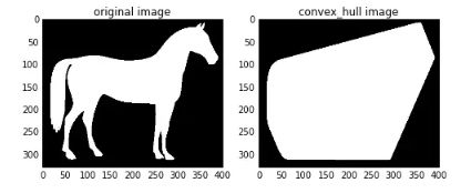

convex_hull_image()是将图片中的所有目标看作一个整体，因此计算出来只有一个最小凸多边形。如果图中有多个目标物体，每一个物体需要计算一个最小凸多边形，则需要使用convex_hull_object（）函数。
函数格式：

skimage.morphology.convex_hull_object(image, neighbors=8)

 

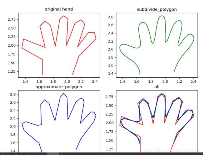
2、 平滑处理

# -*- coding: utf-8 -*-
"""
    Created on 2020/3/5 23:15
    @Author: MGX
    @Description: 
"""
import numpy as np
import matplotlib.pyplot as plt
from skimage import measure,data,color

#生成二值测试图像
hand = np.array([[1.64516129, 1.16145833],
                 [1.64516129, 1.59375],
                 [1.35080645, 1.921875],
                 [1.375, 2.18229167],
                 [1.68548387, 1.9375],
                 [1.60887097, 2.55208333],
                 [1.68548387, 2.69791667],
                 [1.76209677, 2.56770833],
                 [1.83064516, 1.97395833],
                 [1.89516129, 2.75],
                 [1.9516129, 2.84895833],
                 [2.01209677, 2.76041667],
                 [1.99193548, 1.99479167],
                 [2.11290323, 2.63020833],
                 [2.2016129, 2.734375],
                 [2.25403226, 2.60416667],
                 [2.14919355, 1.953125],
                 [2.30645161, 2.36979167],
                 [2.39112903, 2.36979167],
                 [2.41532258, 2.1875],
                 [2.1733871, 1.703125],
                 [2.07782258, 1.16666667]])

#检测所有图形的轮廓
new_hand = hand.copy()
for _ in range(5):
    new_hand =measure.subdivide_polygon(new_hand, degree=2)

# approximate subdivided polygon with Douglas-Peucker algorithm
appr_hand =measure.approximate_polygon(new_hand, tolerance=0.02)

print("Number of coordinates:", len(hand), len(new_hand), len(appr_hand))

fig, axes= plt.subplots(2,2, figsize=(9, 8))
ax0,ax1,ax2,ax3=axes.ravel()

ax0.plot(hand[:, 0], hand[:, 1],'r')
ax0.set_title('original hand')
ax1.plot(new_hand[:, 0], new_hand[:, 1],'g')
ax1.set_title('subdivide_polygon')
ax2.plot(appr_hand[:, 0], appr_hand[:, 1],'b')
ax2.set_title('approximate_polygon')

ax3.plot(hand[:, 0], hand[:, 1],'r')
ax3.plot(new_hand[:, 0], new_hand[:, 1],'g')
ax3.plot(appr_hand[:, 0], appr_hand[:, 1],'b')
ax3.set_title('all')
plt.show()

图例：