基于MNIST数据集的手写体识别
基于MNIST数据集的手写体识别
关于deep learning的第一次实战练习,主要是为了熟悉一下tensorflow的使用。
MNIST数据集
MNIST数据集应该是一个非常经典的深度学习入门训练数据集了。
数据部分,每个图像都是一个28*28的像素点矩阵。
标记部分,是一个10维的向量,数字位为1,非数字位为0。
算法
使用了卷积神经网络(CNN)。
神经网络大概是长这样:卷积层+最大池化层+卷积层+最大池化层+全连接层+输出层
性能评估部分使用了交叉熵作为度量工具。
太菜了,啥都不会,代码基本上是抄tensorflow官方文档的。
代码
import tensorflow as tf
import matplotlib.pyplot as plt
import numpy as np
from tensorflow.examples.tutorials.mnist import input_data
sess=tf.InteractiveSession() #交互流图
mnist=input_data.read_data_sets("MNIST_data", one_hot=True)
#获取数据


def variable_summaries(var):
    with tf.name_scope('summaries'):
      mean = tf.reduce_mean(var)
      tf.summary.scalar('mean', mean)#平均数
      with tf.name_scope('stddev'):
        stddev = tf.sqrt(tf.reduce_mean(tf.square(var - mean)))
      tf.summary.scalar('stddev', stddev)#标准差
      tf.summary.scalar('max', tf.reduce_max(var))#最大
      tf.summary.scalar('min', tf.reduce_min(var))#最小
      tf.summary.histogram('histogram', var)#本身


def weight_variable(shape):
  initial = tf.truncated_normal(shape, stddev=0.1) #正态分布 期望 标准差
  return tf.Variable(initial)
#卷积核初始化

def bias_variable(shape):
  initial=tf.constant(0.1,shape=shape)
  return tf.Variable(initial)
#偏置初始化

def conv2d(x, W):
  return tf.nn.conv2d(x,W,strides=[1,1,1,1],padding='SAME')
#卷积层

def conv2d_reverse(x,W):
  return tf.nn.conv2d_transpose(x,W,strides=[1,1,1,1],padding='SAME')
#可视化 反卷积

def max_pool_2x2(x):
  return tf.nn.max_pool(x,ksize=[1,2,2,1],strides=[1,2,2,1],padding='SAME')
#池化层

def CNN():
  x=tf.placeholder(tf.float32,[None,784])
  y_=tf.placeholder(tf.float32,[None,10])
  with tf.name_scope('input'):
    x_image=tf.reshape(x,[-1,28,28,1])
    tf.summary.image('input', x_image, 5)
  #图像输入

  with tf.name_scope('first_layer'):
    with tf.name_scope('W_conv1'):
      W_conv1=weight_variable([5,5,1,32]) #卷积核 5*5 1通道->32特征
      variable_summaries(W_conv1)
    with tf.name_scope('b_conv1'):
      b_conv1=bias_variable([32]) #偏置矩阵
      variable_summaries(b_conv1)
    h_conv1=tf.nn.relu(conv2d(x_image,W_conv1)+b_conv1) #修正函数,relu=max(0,x)
    h_pool1=max_pool_2x2(h_conv1)

    h_conv1_reverse=conv2d_reverse(x_image,W_conv1)
    tf.summary.image('first_layer', h_conv1_reverse, 5)
    #第一层卷积 卷积层+最大池化层

  W_conv2=weight_variable([5,5,32,64])
  b_conv2=bias_variable([64])
  h_conv2=tf.nn.relu(conv2d(h_pool1,W_conv2)+b_conv2)
  h_pool2=max_pool_2x2(h_conv2)
  #第二层卷积 卷积层+最大池化层

  W_fc1=weight_variable([7*7*64,1024])
  b_fc1=bias_variable([1024])
  h_pool2_flat=tf.reshape(h_pool2,[-1,7*7*64])
  h_fc1=tf.nn.relu(tf.matmul(h_pool2_flat,W_fc1)+b_fc1)
  #全连接层

  keep_prob=tf.placeholder("float")
  h_fc1_drop=tf.nn.dropout(h_fc1,keep_prob)
  #过拟合处理 随机扔掉一些神经元

  W_fc2=weight_variable([1024,10])
  b_fc2=bias_variable([10])
  y_conv=tf.nn.softmax(tf.matmul(h_fc1_drop,W_fc2)+b_fc2)
  #输出层

  with tf.name_scope('loss'):
    cross_entropy=-tf.reduce_sum(y_*tf.log(y_conv))
    tf.summary.scalar('loss',cross_entropy)
  #计算交叉熵
  train_step=tf.train.AdamOptimizer(1e-4).minimize(cross_entropy) #Adam优化算法
  correct_prediction=tf.equal(tf.argmax(y_conv,1),tf.argmax(y_,1)) #比较预测结果与标记 argmax:最大值的索引
  with tf.name_scope('accuracy'):
    accuracy=tf.reduce_mean(tf.cast(correct_prediction,"float"))  #求平均值(准确率) csdt:数据类型转换
    tf.summary.scalar('accuracy',accuracy)
  #性能评估

  sess.run(tf.initialize_all_variables())
  merged=tf.summary.merge_all()
  writer=tf.summary.FileWriter("logs", sess.graph)#将训练日志写到logs文件夹下

  for i in range(2000):
    batch = mnist.train.next_batch(50)
    if i%100 == 0:
      train_accuracy=accuracy.eval(feed_dict={x:batch[0],y_:batch[1],keep_prob:1.0})
      print ('step %d, training accuracy %g'%(i, train_accuracy))
    result,_=sess.run([merged, train_step],feed_dict={x:batch[0],y_:batch[1],keep_prob:0.5})
    writer.add_summary(result,i)

  print ('test accuracy %g'%accuracy.eval(feed_dict={
    x:mnist.test.images,y_:mnist.test.labels, keep_prob:1.0}))
  #test

if __name__ == '__main__':
    CNN()
运行结果
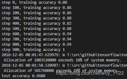
跑若干次,每次取50张图片进行训练。
跑1000次CNN能连到96%
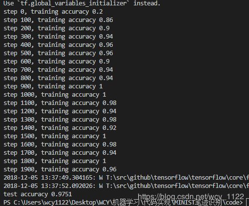
跑2000次CNN能练到97.5%
tensorboard与可视化
tensorboard的使用
使用了tensorboard,让训练结果可视化。
打开终端,运行如下代码,然后打开http://localhost:6006就能看到tensorboard生成的图像了。
tensorboard --logdir path(路径)
tensorboard上的可视化结果
1、损失函数与准确率
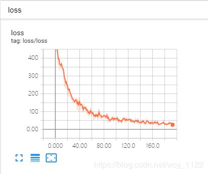
使用交叉熵进行计算的损失函数
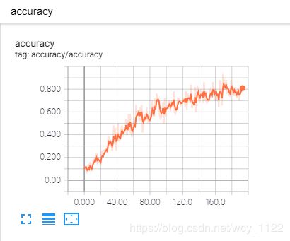
每次训练的训练集的准确率
2、卷积核与偏置矩阵
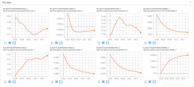
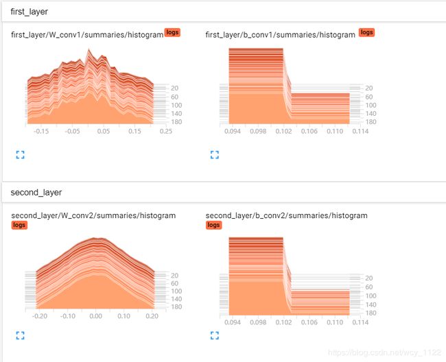
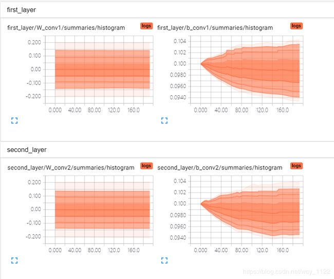
第一层神经网络的卷积核与偏置矩阵
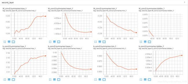 第二层神经网络的卷积核与偏置矩阵
3、基于反卷积的图像输出
加入的反卷积函数,通过反卷积得到每层神经网络后的图像。
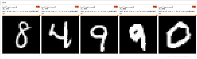
输入图像
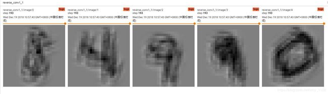
第一层卷积后的图像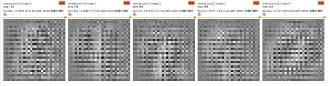
第二层卷积后的图像
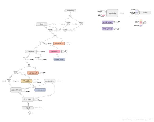
4、流图