配准中雅可比行列式（Jacobian determinant）的原理、意义、代码实现以及可视化（5.14更新）

• 2020-2-23更新

网友芒果和小猫通过评论分享了解释行列式的对角线元素+1的原因，参见该网址，我们将原文引用如下，并简单翻译解释：

原文如下：

Note that the determinant of a zero vector field is also zero, whereas the Jacobian determinant of the corresponding identity warp transformation is 1.0. In order to compute the effective deformation Jacobian determinant 1.0 must be added to the diagonal elements of Jacobian prior to taking the derivative. i.e. det([ (1.0+dx/dx) dx/dy dx/dz ; dy/dx (1.0+dy/dy) dy/dz; dz/dx dz/dy (1.0+dz/dz) ])

解释如下：

值得注意的是，零位移矢量场的行列式的值为0，然而相应的恒等变换（即对原图进行变形后的图像，仍与原图相同）的雅克比行列式的值为1。因此，为了计算出有效的变形场的雅克比行列式，在求导之前要再雅克比式的对角线元素上加1，使得数学计算的结果与实际相符。

---

• 2019-5-14更新

最近两天我研究了一下雅可比行列式的问题，重新检查了别人的公开代码与可视化，发现了一些问题，现总结如下：

1. 检查雅可比行列式的计算原理与其代码实现，我发现之前的代码存在问题，现在进行更新纠正；
2. 关于其代码实现，我还有一个疑问没有解答，这可能与其数学原理有关，需要进一步的验证；
3. 对雅可比行列式的计算结果进行可视化，本文提供了代码参考，并进行了解释，但还没解决。

1.正确的代码实现

用代码来计算雅可比行列式，实际上就是将这个三阶行列式进行展开。参照行列式展开的结果，我检查github上的公开代码（参见更新前的代码），发现其中存在一个错误和两个问题。首先小错误是在D2的计算中，D_x[...,0]实际上应该为D_z[...,0]；其中一个问题是在计算最终结果时，它取了绝对值（np.abs()），也就是说，它完全忽视了负值的情况，这就减少了其可视化的工作量，但也损失了最重要的信息。另外一个问题参见第二小节（2.代码实现的一个疑问）。

如下是我修改后的代码，以及注释：

def Get_Jac(displacement):
    '''
    the expected input: displacement of shape(batch, H, W, D, channel),
    obtained in TensorFlow.
    '''
    D_y = (displacement[:,1:,:-1,:-1,:] - displacement[:,:-1,:-1,:-1,:])
    D_x = (displacement[:,:-1,1:,:-1,:] - displacement[:,:-1,:-1,:-1,:])
    D_z = (displacement[:,:-1,:-1,1:,:] - displacement[:,:-1,:-1,:-1,:])

    D1 = (D_x[...,0]+1)*((D_y[...,1]+1)*(D_z[...,2]+1) - D_y[...,2]*D_z[...,1])
    D2 = (D_x[...,1])*(D_y[...,0]*(D_z[...,2]+1) - D_y[...,2]*D_z[...,0])
    D3 = (D_x[...,2])*(D_y[...,0]*D_z[...,1] - (D_y[...,1]+1)*D_z[...,0])
    
    D = D1 - D2 + D3
    
    return D

2.代码实现的一个疑问

对比行列式展开与以上的代码实现，可以发现，在计算D1,D2,D3时，中间出现了+1的情况，而且是行列式的对角线元素+1。由于我没有查阅关于雅可比行列式的原始文献，不清楚代码的原始作者这样做的具体原因。我猜测，这或许与其数学原理有关，可能与其物理意义相对应（当其值为1时该点的形状保持不变）。需要指出的是，该代码还没经过验证，不一定就是正确的计算方法。据了解，simpleitk 或者simpleelastix上可能有相关的计算，可以与之进行结果对比。

该疑问的解释，请查看2020-2-23更新内容。

3.可视化

在github上相同repository的visual.py中，可以找到关于雅可比式的可视化代码，并尝试用其绘制了一些图，参考了文件中注释掉的绘图代码。需要特别注意的是，MidpointNormalize类是作者从matplotlib中的实例中抄录过来的。它是将矩阵中的所有元素根据用户指定的最小值、中间点（midpoint）、最大值分别与【0,0.5,1】对应，进行两段线性映射，将所有值映射到【0,1】。这里涉及到绘图的细节方面，就不再赘述。

可视化代码：

"""
Created on Wed Apr 11 10:08:36 2018
@author: Dongyang
This script contains some utilize functions for data visualization
"""
import matplotlib.pyplot as plt
from matplotlib import colors
import numpy as np

#==============================================================================
# Define a custom colormap for visualiza Jacobian
#==============================================================================
class MidpointNormalize(colors.Normalize):
    def __init__(self, vmin=None, vmax=None, midpoint=None, clip=False):
        self.midpoint = midpoint
        colors.Normalize.__init__(self, vmin, vmax, clip)

    def __call__(self, value, clip=None):
        # I'm ignoring masked values and all kinds of edge cases to make a
        # simple example...
        x, y = [self.vmin, self.midpoint, self.vmax], [0, 0.5, 1]
        return np.ma.masked_array(np.interp(value, x, y))

#==============================================================================
# plot an array of images for comparison
#==============================================================================    
def show_sample_slices(sample_list,name_list, Jac = False, cmap = 'gray', attentionlist=None):
  num = len(sample_list)
  fig, ax = plt.subplots(1,num)
  for i in range(num):
    if Jac:
        ax[i].imshow(sample_list[i], cmap, norm=MidpointNormalize(midpoint=1))
    else:
        ax[i].imshow(sample_list[i], cmap)
    ax[i].set_title(name_list[i])
    ax[i].axis('off')
    if attentionlist:
        ax[i].add_artist(attentionlist[i])
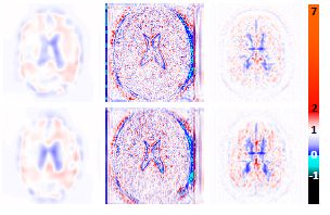
  plt.subplots_adjust(wspace=0)

调用以上代码，我利用胸部图像的形变场绘制了下面的图像，并加上了colorbar。问题是，该图像中没有显示负值的情况。此处还需要进一步的研究与完善。如果有什么问题与错误，期待各位网友的批评指正。

---

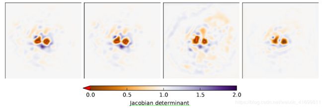
引言

在医学图像配准的文章中经常会看到类似下面的图，它是什么，代表什么含义呢？本文的目的就是给大家分享一下其数学原理与实际意义。

介绍

上图是雅可比矩阵的可视化结果，而其中的每一个元素为雅可比式（即雅可比行列式，Jacobian determinant）。通常，配准后，我们会得到图像的变形场(deformation field)，即图像的每个像素的位移组成的场，简称为密集位移场（dense displacement vector field, DVF）。通过对DVF进行评价来验证配准方法的特性， 而雅可比矩阵就是评估DVF的拓扑特性的一种常用指标。

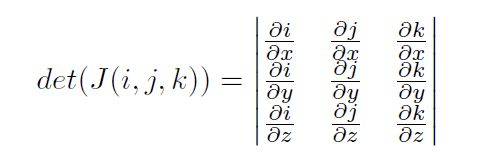
原理

雅可比式的定义，以三维数据为例，即在DVF上的每个点p(i, j, k)上

当其值=1时，在该点处的体积没有发生变化；>1时，发生膨胀；在0-1之间时，发生缩小；<=0时，为奇点，意味着图像在该点出现折叠现象。通过计算每幅图的折叠百分数和雅可比式的标准差，我们可以量化DVF的质量，指其的拓扑特性。

意义

由于图像折叠（folding）在解剖学上是不太可能的，特别是在同一个病人的图像之间进行配准，我们可以定量评估配准后得到的DVF的拓扑结构，或者是可视化雅可比矩阵，来验证配准是否出现了折叠，以此判断配准结果的优劣。

代码

import numpy as np

#==============================================================================
# Calculate the Determinent of Jacobian of the transformation
#==============================================================================

def Get_Ja(displacement):

    '''
    '''
  
    D_y = (displacement[:,1:,:-1,:-1,:] - displacement[:,:-1,:-1,:-1,:])
    D_x = (displacement[:,:-1,1:,:-1,:] - displacement[:,:-1,:-1,:-1,:])
    D_z = (displacement[:,:-1,:-1,1:,:] - displacement[:,:-1,:-1,:-1,:])
  
    D1 = (D_x[...,0]+1)*( (D_y[...,1]+1)*(D_z[...,2]+1) - D_z[...,1]*D_y[...,2])
    D2 = (D_x[...,1])*(D_y[...,0]*(D_z[...,2]+1) - D_y[...,2]*D_x[...,0])
    D3 = (D_x[...,2])*(D_y[...,0]*D_z[...,1] - (D_y[...,1]+1)*D_z[...,0])
    D = np.abs(D1-D2+D3)

    return D

参考文献

1. 左图及原理  Bob D. de Vos, Floris F. Berendsen, Max A. Viergever and et al. A Deep Learning Framework for Unsupervised
Affine and Deformable Image Registration. Preprint submitted to Medical Image Analysis. arXiv:1809.06130v1 [cs.CV] 2018

2. 右图 J. Krebs , T. Mansi, B. Mailh´e, N. Ayache, and H. Delingette. Learning Structured Deformations using Diffeomorphic Regsitration. arXiv:1804.07172v1 [cs.CV], 2018. 

3. 代码 https://github.com/dykuang/Medical-image-registration/blob/master/source/Utils.py