从零单排入门机器学习：线性回归（linear regression）实践篇

     线性回归（linear regression）实践篇

之前一段时间在coursera看了Andrew ng的机器学习的课程，感觉还不错，算是入门了。这次打算以该课程的作业为主线，对机器学习基本知识做一下总结。小弟才学疏浅，如有错误，敬请指导。

问题原描述：

you will implement linear regression with one
variable to predict prots for a food truck. Suppose you are the CEO of a
restaurant franchise and are considering dierent cities for opening a new
outlet. The chain already has trucks in various cities and you have data for
prots and populations from the cities.

简单来说，就是根据一个城市的人口数量，来预测一辆快餐车能获得的利益。

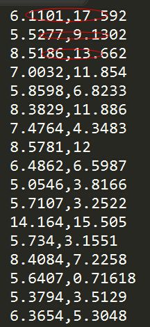
数据集大概是这样子的：

一行数据为一个样本。第一列表示人口，第二列表示利益。

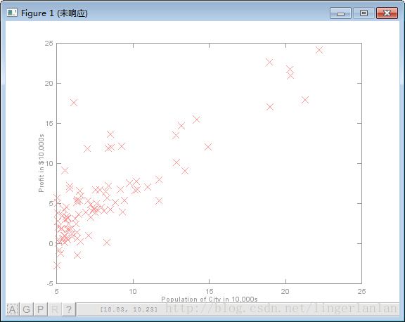
首先，先把数据可视化。

%% ======================= Part 2: Plotting =======================
fprintf('Plotting Data ...\n')
data = load('ex1data1.txt');
X = data(:, 1); y = data(:, 2);
m = length(y); % number of training examples

% Plot Data
% Note: You have to complete the code in plotData.m
plotData(X, y);

fprintf('Program paused. Press enter to continue.\n');
pause;

function plotData(x, y)
%PLOTDATA Plots the data points x and y into a new figure 
%   PLOTDATA(x,y) plots the data points and gives the figure axes labels of
%   population and profit.

% ====================== YOUR CODE HERE ======================
% Instructions: Plot the training data into a figure using the 
%               "figure" and "plot" commands. Set the axes labels using
%               the "xlabel" and "ylabel" commands. Assume the 
%               population and revenue data have been passed in
%               as the x and y arguments of this function.
%
% Hint: You can use the 'rx' option with plot to have the markers
%       appear as red crosses. Furthermore, you can make the
%       markers larger by using plot(..., 'rx', 'MarkerSize', 10);

figure; % open a new figure window

plot(x, y, 'rx', 'MarkerSize', 10); % Plot the data
ylabel('Profit in $10,000s'); % Set the y label
xlabel('Population of City in 10,000s'); % Set the x label





% ============================================================

end

计算cost function

function J = computeCost(X, y, theta)
%COMPUTECOST Compute cost for linear regression
%   J = COMPUTECOST(X, y, theta) computes the cost of using theta as the
%   parameter for linear regression to fit the data points in X and y

% Initialize some useful values
m = length(y); % number of training examples

% You need to return the following variables correctly 
% ====================== YOUR CODE HERE ======================
% Instructions: Compute the cost of a particular choice of theta
%               You should set J to the cost.
H = X*theta;
diff = H - y;
%J = sum(diff.^2)/(2*m);
J = sum(diff.*diff)/(2*m);

% =========================================================================

end

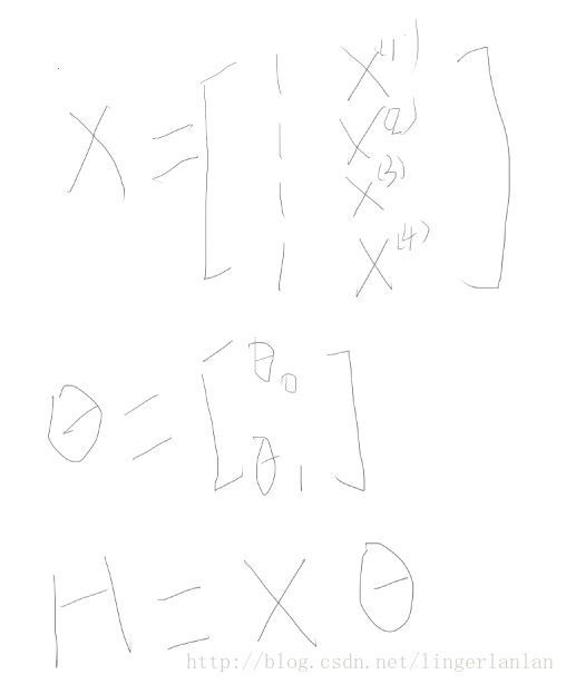
为了方便理解上面代码，看看各变量大概长什么样子的。

梯度下降法计算参数theta

function [theta, J_history] = gradientDescent(X, y, theta, alpha, num_iters)
%GRADIENTDESCENT Performs gradient descent to learn theta
%   theta = GRADIENTDESENT(X, y, theta, alpha, num_iters) updates theta by 
%   taking num_iters gradient steps with learning rate alpha

% Initialize some useful values
m = length(y); % number of training examples
J_history = zeros(num_iters, 1);

for iter = 1:num_iters

    % ====================== YOUR CODE HERE ======================
    % Instructions: Perform a single gradient step on the parameter vector
    %               theta. 
    %
    % Hint: While debugging, it can be useful to print out the values
    %       of the cost function (computeCost) and gradient here.
    %

    H = X*theta-y;
    theta(1) = theta(1) - sum(H.* X(:,1))*alpha/m;%感觉这样写挺搓的
    theta(2) = theta(2) - sum(H.* X(:,2))*alpha/m;
    %theta = theta - alpha * (X' * (X * theta - y)) / m; 


    % ============================================================

    % Save the cost J in every iteration    
    J_history(iter) = computeCost(X, y, theta);

end

end

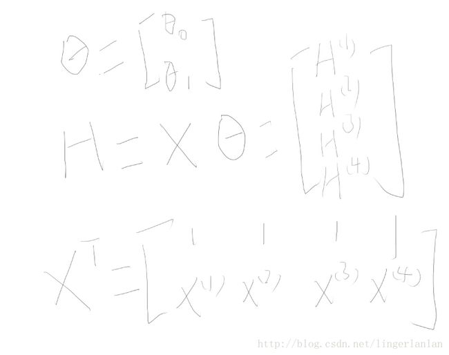
难以理解的是theta = theta - alpha * (X' * (X * theta - y)) / m; 这种向量化算法。

先看看theta本质是怎么计算的

再看看各变量长什么样子的

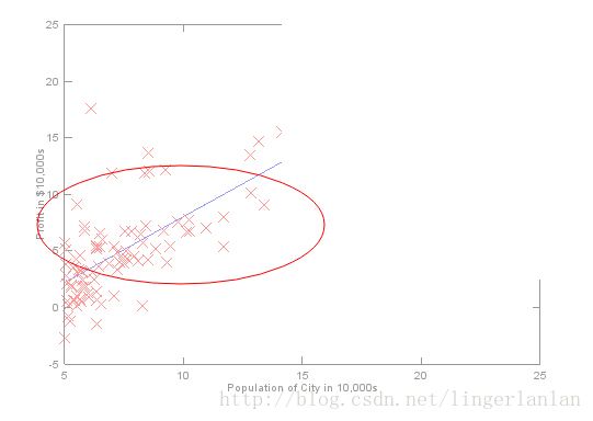
算出theta之后，就可以画出拟合直线了。

注：本文作者linger，如有转载，请标明转载于http://blog.csdn.net/lingerlanlan。

本文链接:http://blog.csdn.net/lingerlanlan/article/details/32162559