机器学习案例实战：交易数据异常检测

原创文章,如需转载请保留出处
本博客为唐宇迪老师python数据分析与机器学习实战课程学习笔记

一. 案例背景目标
1.1 背景
现给定一些信用卡相关数据，从中剔除异常数据

import pandas as pd
import matplotlib.pyplot as plt
import numpy as np
%matplotlib inline

data = pd.read_csv('creditcard.csv')
data.head()
data.shape

(284807, 31)
数据共284807行，31列

	Time	V1	V2	V3	V4	V5	V6	V7	V8	V9	...	V21	V22	V23	V24	V25	V26	V27	V28	Amount	Class
0	0.0	-1.359807	-0.072781	2.536347	1.378155	-0.338321	0.462388	0.239599	0.098698	0.363787	...	-0.018307	0.277838	-0.110474	0.066928	0.128539	-0.189115	0.133558	-0.021053	149.62	0
1	0.0	1.191857	0.266151	0.166480	0.448154	0.060018	-0.082361	-0.078803	0.085102	-0.255425	...	-0.225775	-0.638672	0.101288	-0.339846	0.167170	0.125895	-0.008983	0.014724	2.69	0
2	1.0	-1.358354	-1.340163	1.773209	0.379780	-0.503198	1.800499	0.791461	0.247676	-1.514654	...	0.247998	0.771679	0.909412	-0.689281	-0.327642	-0.139097	-0.055353	-0.059752	378.66	0
3	1.0	-0.966272	-0.185226	1.792993	-0.863291	-0.010309	1.247203	0.237609	0.377436	-1.387024	...	-0.108300	0.005274	-0.190321	-1.175575	0.647376	-0.221929	0.062723	0.061458	123.50	0
4	2.0	-1.158233	0.877737	1.548718	0.403034	-0.407193	0.095921	0.592941	-0.270533	0.817739	...	-0.009431	0.798278	-0.137458	0.141267	-0.206010	0.502292	0.219422	0.215153	69.99	0
5 rows × 31 columns

二.样本不均衡解决方案
2.1 统计数据

#分别统计0和1个数
count_classes = pd.value_counts(data['Class'],sort = True).sort_index()
print(count_classes)
#画图显示统计个数
count_classes.plot(kind='bar')
plt.title("Fraud class histogram")
plt.xlabel("Class")
plt.ylabel("Frequency")

0 284315（正常数据）
1 492（异常数据）
Name: Class, dtype: int64

2.2 两种采样策略

• 下采样：正常数据284315条，异常数据492条。从正常数据中取和异常数据一样多的数据。
• 过采样：正常数据284315条，异常数据492条。在异常数据生成和正常数据一样多的数据。

2.3 对数据预处理

#导入sklearn下预处理模块preprocessing
from sklearn.preprocessing import StandardScaler
#fit_transform对数据进行变换操作（不仅计算训练数据的均值和方差，还会基于计算出来的均值和方差来转换训练数据，从而把数据转换成标准的正太分布）
data['normAmount'] = StandardScaler().fit_transform(data['Amount'].values.reshape(-1, 1))
data = data.drop(['Time','Amount'],axis=1)
data.head()

	V1	V2	V3	V4	V5	V6	V7	V8	V9	V10	...	V21	V22	V23	V24	V25	V26	V27	V28	Class	normAmount
0	-1.359807	-0.072781	2.536347	1.378155	-0.338321	0.462388	0.239599	0.098698	0.363787	0.090794	...	-0.018307	0.277838	-0.110474	0.066928	0.128539	-0.189115	0.133558	-0.021053	0	0.244964
1	1.191857	0.266151	0.166480	0.448154	0.060018	-0.082361	-0.078803	0.085102	-0.255425	-0.166974	...	-0.225775	-0.638672	0.101288	-0.339846	0.167170	0.125895	-0.008983	0.014724	0	-0.342475
2	-1.358354	-1.340163	1.773209	0.379780	-0.503198	1.800499	0.791461	0.247676	-1.514654	0.207643	...	0.247998	0.771679	0.909412	-0.689281	-0.327642	-0.139097	-0.055353	-0.059752	0	1.160686
3	-0.966272	-0.185226	1.792993	-0.863291	-0.010309	1.247203	0.237609	0.377436	-1.387024	-0.054952	...	-0.108300	0.005274	-0.190321	-1.175575	0.647376	-0.221929	0.062723	0.061458	0	0.140534
4	-1.158233	0.877737	1.548718	0.403034	-0.407193	0.095921	0.592941	-0.270533	0.817739	0.753074	...	-0.009431	0.798278	-0.137458	0.141267	-0.206010	0.502292	0.219422	0.215153	0	-0.073403
5 rows × 30 columns

三.下采样策略
3.1 根据下采样策略生成样本

#找不包括Class列的数据
X = data.loc[:, data.columns != 'Class']
#找只包括Class列的数据
y = data.loc[:, data.columns == 'Class']

#让数据等于0的个数和等于1的个数一样少
#class等于1的个数
number_records_fraud = len(data[data.Class == 1])
#class等于1的索引
fraud_indices = np.array(data[data.Class == 1].index)

#class等于0的索引
normal_indices = data[data.Class == 0].index

#np.random.choice 随机选择
#参数：从正常索引里(normal_indices)选取异常的个数(number_records_fraud)，replace表示是否可以重用元素，默认为False
random_normal_indices = np.random.choice(normal_indices, number_records_fraud, replace = False)
#转换成数组
random_normal_indices = np.array(random_normal_indices)

#合并两种索引
under_sample_indices = np.concatenate([fraud_indices,random_normal_indices])

#把只有索引值转换成data格式
under_sample_data = data.iloc[under_sample_indices,:]

#把under_sample_data分成两种格式
X_undersample = under_sample_data.loc[:, under_sample_data.columns != 'Class']
y_undersample = under_sample_data.loc[:, under_sample_data.columns == 'Class']

print("Percentage of normal transactions: ", len(under_sample_data[under_sample_data.Class == 0])/len(under_sample_data))
print("Percentage of fraud transactions: ", len(under_sample_data[under_sample_data.Class == 1])/len(under_sample_data))
print("Total number of transactions in resampled data: ", len(under_sample_data))

Percentage of normal transactions: 0.5
Percentage of fraud transactions: 0.5
Total number of transactions in resampled data: 984
​
四.交叉验证
4.1 交叉验证理解

1. 拿到一组数据，选择其中80%当训练数据，建立模型。剩下20%当测试数据验证这个模型。
2. 在训练集上平均切除三分，用这三分数据进行交叉验证：
   - (1) 用一号和二号训练集建立模型，用三号训练集验证当前模型下的参数
   - (2) 用一号和三号训练集建立模型，用二号训练集验证当前模型下的参数
   - (3) 用二号和三号训练集建立模型，用一号训练集验证当前模型下的参数
   为什么这么做？目的是为了求稳，让模型的评估效果是可信的，三个训练集都有评估的标准，让其平均值作为衡量模型效果

4.2 对数据切分

from sklearn.model_selection import train_test_split
#对元素数据集切分
#test_size:切分比例，30%测试集，70%训练集
#random_state:先洗牌，再切分
X_train, X_test, y_train, y_test = train_test_split(X,y,test_size = 0.3, random_state = 0)

print("Number transactions train dataset:", len(X_train))
print("Number transactions test dataset:", len(X_test))
print("Total number of transactions:", len(X_train)+len(X_test))

#对下采样数据集切分
X_train_undersample, X_test_undersample, y_train_undersample, y_test_undersample = train_test_split(X_undersample,y_undersample,test_size = 0.3,random_state = 0)

print("Number transactions train dataset:", len(X_train_undersample))
print("Number transactions test dataset:", len(X_test_undersample))
print("Total number of transactions:", len(X_train_undersample)+len(X_test_undersample))

Number transactions train dataset: 199364
Number transactions test dataset: 85443
Total number of transactions: 284807
Number transactions train dataset: 688
Number transactions test dataset: 296
Total number of transactions: 984

五.模型评估方法
5.1 召回率(Recall)
召回率是覆盖面的度量，度量有多个正例被分为正例
Recall = TP/(TP+FN)

5.2 举个例子
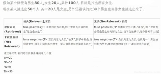
假设我们手上有60个正样本，40个负样本，我们要找出所有的正样本，系统查找出50个，其中只有40个是真正的正样本，计算上述各指标。

TP: 将正类预测为正类数 40
FN: 将正类预测为负类数 20（60-40个是真正的正样本）
FP: 将负类预测为正类数 10（50-40个是真正的正样本）
TN: 将负类预测为负类数 30（40个负样 -（50-40个是真正的正样本））

准确率(accuracy) = 预测对的/所有 = (TP+TN)/(TP+FN+FP+TN) = 70%
精确率(precision) = TP/(TP+FP) = 80%
召回率(recall) = TP/(TP+FN) = 2/3

六.正交化惩罚
逻辑回归中，其实有些参数需要指定。如正则化惩罚项
6.1 什么是正则化
假设求逻辑回归，A模型(θ1···θ10)，B模型(θ1···θ10)。虽然A和B内θ都不一样，A模型θ浮动比较大，B模型θ浮动比较小，但Recall都是90%

• 我们希望获取浮动较小的模型，因为浮动较小，过拟合的风险较小。(过拟合：模型在训练集上效果表现较好，在测试集上效果表现不好)
• 我们希望得到B模型，如何得到B模型呢？
  引入正则化惩罚，希望能大力度的惩罚A模型，小力度的惩罚B模型
  如：L2正则化
  L2正则化：在目标函数(损失函数)加上1/2W²
  即，loss+1/2W²
  A模型的浮动大，则W²更大，B模型W²小，虽然两个模型Recall值是一样的，但通过计算loss+1/2W²，比较哪个模型效果更好。
  附：L1正则化：在目标函数(损失函数)加上|W|
• 引入惩罚力度（λ）
  λL2
  通过控制λ，调整惩罚力度

七.逻辑回归模型
7.1 模型的评估标准

def printing_Kfold_scores(x_train_data,y_train_data):
    #先传入原始数据len(y_train_data)，再做5倍的交叉验证
    fold = KFold(5,shuffle=False)
    
    c_param_range = [0.01,0.1,1,10,100]
    
    results_table = pd.DataFrame(index = range(len(c_param_range),2), columns = ['C_paramter','Mean recall score'])
    results_table['C_parameter'] = c_param_range
    
    j = 0
    #循环c_param_range，比较哪个值好
    for c_param in c_param_range:
        print('----------------------------------------')
        print('C_parameter:' , c_param)
        print('----------------------------------------')
        print('')
        
        recall_accs = []
        #循环交叉验证
        for iteration, indices in enumerate(fold.split(x_train_data)):
            #C：惩罚力度
            #penalty：选择哪种惩罚l1或l2
            lr = LogisticRegression(C = c_param, penalty = 'l1')
            
            #fit:交叉验证，建立模型
            lr.fit(x_train_data.iloc[indices[0],:],y_train_data.iloc[indices[0],:].values.ravel())
              
            y_pred_undersample = lr.predict(x_train_data.iloc[indices[1],:].values)  
            recall_acc = recall_score(y_train_data.iloc[indices[1],:].values,y_pred_undersample) 
            recall_accs.append(recall_acc)
            print('Iteration',iteration,': recall score = ', recall_acc)
        results_table.loc[j,'Mean recall score'] = np.mean(recall_accs)
        j += 1
        print('')
        print('Mean recall score', np.mean(recall_accs))
        print('')
    best_c=results_table.loc[results_table['Mean recall score'].astype('float64').idxmax()]['C_parameter']
    print('*****************************************************************')
    print('Best model to choose from cross validation is with C parameter = ', best_c)
    print('*****************************************************************')
    return best_c

best_c=printing_Kfold_scores(X_train_undersample,y_train_undersample)

---

C_parameter: 0.01

Iteration 0 : recall score = 0.9315068493150684
Iteration 1 : recall score = 0.9178082191780822
Iteration 2 : recall score = 1.0
Iteration 3 : recall score = 0.9459459459459459
Iteration 4 : recall score = 0.9696969696969697

Mean recall score 0.9529915968272131

---

C_parameter: 0.1

Iteration 0 : recall score = 0.8493150684931506
Iteration 1 : recall score = 0.863013698630137
Iteration 2 : recall score = 0.9491525423728814
Iteration 3 : recall score = 0.9459459459459459
Iteration 4 : recall score = 0.9090909090909091

Mean recall score 0.9033036329066049

---

C_parameter: 1

Iteration 0 : recall score = 0.863013698630137
Iteration 1 : recall score = 0.8904109589041096
Iteration 2 : recall score = 0.9830508474576272
Iteration 3 : recall score = 0.9459459459459459
Iteration 4 : recall score = 0.9090909090909091

Mean recall score 0.9183024720057457

---

C_parameter: 10

Iteration 0 : recall score = 0.863013698630137
Iteration 1 : recall score = 0.8904109589041096
Iteration 2 : recall score = 0.9830508474576272
Iteration 3 : recall score = 0.9324324324324325
Iteration 4 : recall score = 0.9090909090909091

Mean recall score 0.9155997693030431

---

C_parameter: 100

Iteration 0 : recall score = 0.8904109589041096
Iteration 1 : recall score = 0.9041095890410958
Iteration 2 : recall score = 0.9830508474576272
Iteration 3 : recall score = 0.9459459459459459
Iteration 4 : recall score = 0.9090909090909091

Mean recall score 0.9265216500879376

---

Best model to choose from cross validation is with C parameter = 0.01

---

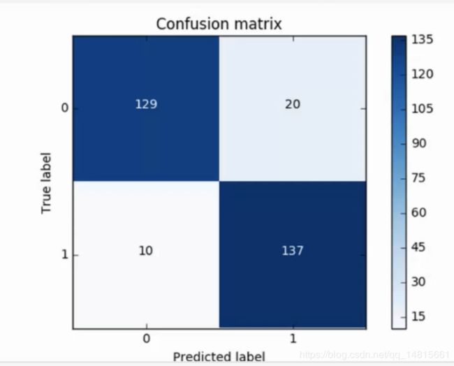
八.混淆矩阵
8.1 下采样数据集的混淆矩阵

8.2 原始数据集的混淆矩阵

#原始数据，不带下采样
best_c=printing_Kfold_scores(X_train,y_train)

----------------------------------------
C_parameter: 0.01
----------------------------------------

Iteration 0 : recall score =  0.4925373134328358
Iteration 1 : recall score =  0.6027397260273972
Iteration 2 : recall score =  0.6833333333333333
Iteration 3 : recall score =  0.5692307692307692
Iteration 4 : recall score =  0.45

Mean recall score 0.5595682284048672

----------------------------------------
C_parameter: 0.1
----------------------------------------

Iteration 0 : recall score =  0.5671641791044776
Iteration 1 : recall score =  0.6164383561643836
Iteration 2 : recall score =  0.6833333333333333
Iteration 3 : recall score =  0.5846153846153846
Iteration 4 : recall score =  0.525

Mean recall score 0.5953102506435158

----------------------------------------
C_parameter: 1
----------------------------------------

Iteration 0 : recall score =  0.5522388059701493
Iteration 1 : recall score =  0.6164383561643836
Iteration 2 : recall score =  0.7166666666666667
Iteration 3 : recall score =  0.6153846153846154
Iteration 4 : recall score =  0.5625

Mean recall score 0.612645688837163

----------------------------------------
C_parameter: 10
----------------------------------------

Iteration 0 : recall score =  0.5522388059701493
Iteration 1 : recall score =  0.6164383561643836
Iteration 2 : recall score =  0.7333333333333333
Iteration 3 : recall score =  0.6153846153846154
Iteration 4 : recall score =  0.575

Mean recall score 0.6184790221704963

----------------------------------------
C_parameter: 100
----------------------------------------

Iteration 0 : recall score =  0.5522388059701493
Iteration 1 : recall score =  0.6164383561643836
Iteration 2 : recall score =  0.7333333333333333
Iteration 3 : recall score =  0.6153846153846154
Iteration 4 : recall score =  0.575

Mean recall score 0.6184790221704963

*****************************************************************
Best model to choose from cross validation is with C parameter =  10.0
*****************************************************************

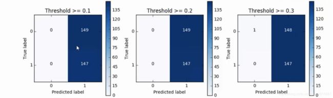
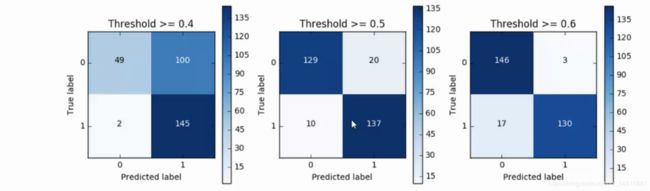
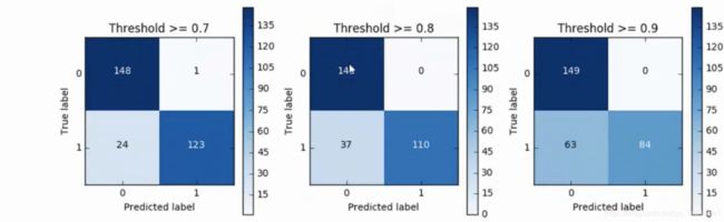
九.逻辑回归阈值对结果的影响



十.SMOTE样本生成策略