(R语言)风电机组运行数据分析
风电机组运行数据分析
基于R语言,对德国某风电场7台850kw的风电机组运行数据进行分析。约5万条数据。
部分数据:
读取数据:
> data <- read.csv(file.choose())
> head(data)
  PCTimeStamp
1      1/1/13
2 1/1/13 0:10
3 1/1/13 0:20
4 1/1/13 0:30
5 1/1/13 0:40
6 1/1/13 0:50
  WTG01_Grid.Production.PossiblePower.Avg...1.
1                                          817
2                                          732
3                                          764
4                                          773
5                                          689
6                                          735
  WTG02_Grid.Production.PossiblePower.Avg...2.
1                                          805
2                                          790
3                                          774
4                                          769
5                                          690
6                                          753
  WTG03_Grid.Production.PossiblePower.Avg...3.
1                                          786
2                                          763
3                                          793
4                                          759
5                                          711
6                                          808
  WTG04_Grid.Production.PossiblePower.Avg...4.
1                                          809
2                                          809
3                                          821
4                                          813
5                                          800
6                                          830
  WTG05_Grid.Production.PossiblePower.Avg...5.
1                                          755
2                                          771
3                                          736
4                                          627
5                                          749
6                                          832
  WTG06_Grid.Production.PossiblePower.Avg...6.
1                                          745
2                                          758
3                                          668
4                                          717
5                                          749
6                                          757
  WTG07_Grid.Production.PossiblePower.Avg...7.
1                                          743
2                                          811
3                                          656
4                                          752
5                                          723
6                                          797
  WTG01_Total.Active.power..8.
1                      3109970
2                      3110050
3                      3110130
4                      3110211
5                      3110288
6                      3110366
  WTG02_Total.Active.power..9.
1                       609852
2                       609933
3                       610014
4                       610095
5                       610176
6                       610257
  WTG03_Total.Active.power..10.
1                       3254759
2                       3254839
3                       3254920
4                       3255002
5                       3255083
6                       3255164
  WTG04_Total.Active.power..11.
1                       3341303
2                       3341384
3                       3341465
4                       3341546
5                       3341628
6                       3341709
  WTG05_Total.Active.power..12.
1                       3230186
2                       3230266
3                       3230346
4                       3230421
5                       3230501
6                       3230582
  WTG06_Total.Active.power..13.
1                       3264175
2                       3264255
3                       3264336
4                       3264417
5                       3264499
6                       3264579
  WTG07_Total.Active.power..14.
1                       3136754
2                       3136835
3                       3136914
4                       3136994
5                       3137075
6                       3137156
  MET_Avg..Wind.speed.1..15.
1                       11.3
2                       12.0
3                       11.6
4                       11.8
5                       11.2
6                       11.1
  MET_Min..Wind.speed.1..16.
1                        8.1
2                        9.1
3                        7.1
4                        9.4
5                        8.1
6                        7.1
  MET_Max..Wind.speed.1..17. GRID1_KWH_DEL
1                       14.5       2510065
2                       15.4       2510615
3                       16.7       2511165
4                       14.2       2511714
5                       14.3       2512265
6                       14.4       2512815
更改列名:
> new.names<-c("date_time","T1_Possible_Power","T2_Possible_Power","T3_Possible_Power","T4_Possible_Power","T5_Possible_Power","T6_Possible_Power","T7_Possible_Power","T1_Total_Active_Power","T2_Total_Active_Power","T3_Total_Active_Power","T4_Total_Active_Power","T5_Total_Active_Power","T6_Total_Active_Power","T7_Total_Active_Power","mean_wind_mps", "min_wind_mps", "max_wind_mps", "cum_energy_delivered_kwh")> cbind(names(data),new.names)
> names(data) <- new.names按类型划分子集数据:
大多数时候我们只需要累计的能量和风速相关的数据。
Cumulative<-subset(data, select=c(1,19))
Possible<-subset(data, select=1:8)
Active<-subset(data, select=c(1,9:15))
Wind<-subset(data, select=c(1,16:18))dat<-data数据统计性描述:
1、数据维度:
> dim(dat)
[1] 52560 192、数据类型:
> str(dat)
'data.frame':	52560 obs. of  19 variables:
 $ date_time               : Factor w/ 52560 levels "1/1/13","1/1/13 0:10",..: 1 2 3 4 5 6 7 8 9 10 ...
 $ T1_Possible_Power       : int  817 732 764 773 689 735 782 814 730 727 ...
 $ T2_Possible_Power       : int  805 790 774 769 690 753 818 796 735 773 ...
 $ T3_Possible_Power       : int  786 763 793 759 711 808 736 789 736 768 ...
 $ T4_Possible_Power       : int  809 809 821 813 800 830 822 835 805 832 ...
 $ T5_Possible_Power       : int  755 771 736 627 749 832 713 747 780 797 ...
 $ T6_Possible_Power       : int  745 758 668 717 749 757 638 696 716 749 ...
 $ T7_Possible_Power       : int  743 811 656 752 723 797 654 736 683 799 ...
 $ T1_Total_Active_Power   : int  3109970 3110050 3110130 3110211 3110288 3110366 3110447 3110527 3110604 3110682 ...
 $ T2_Total_Active_Power   : int  609852 609933 610014 610095 610176 610257 610338 610419 610499 610579 ...
 $ T3_Total_Active_Power   : int  3254759 3254839 3254920 3255002 3255083 3255164 3255244 3255325 3255406 3255487 ...
 $ T4_Total_Active_Power   : int  3341303 3341384 3341465 3341546 3341628 3341709 3341790 3341870 3341952 3342033 ...
 $ T5_Total_Active_Power   : int  3230186 3230266 3230346 3230421 3230501 3230582 3230662 3230742 3230823 3230904 ...
 $ T6_Total_Active_Power   : int  3264175 3264255 3264336 3264417 3264499 3264579 3264660 3264740 3264821 3264902 ...
 $ T7_Total_Active_Power   : int  3136754 3136835 3136914 3136994 3137075 3137156 3137234 3137314 3137394 3137474 ...
 $ mean_wind_mps           : num  11.3 12 11.6 11.8 11.2 11.1 12 11.3 11.9 11.2 ...
 $ min_wind_mps            : num  8.1 9.1 7.1 9.4 8.1 7.1 9 6.9 8.6 7.9 ...
 $ max_wind_mps            : num  14.5 15.4 16.7 14.2 14.3 14.4 14.8 14.5 15.5 14.8 ...
 $ cum_energy_delivered_kwh: int  2510065 2510615 2511165 2511714 2512265 2512815 2513365 2513915 2514465 2515015 ...
3、数据统计摘要(分位数):
> summary(dat)
       date_time     T1_Possible_Power
 1/1/13     :    1   Min.   : -3.0
 1/1/13 0:10:    1   1st Qu.:191.0
 1/1/13 0:20:    1   Median :518.0
 1/1/13 0:30:    1   Mean   :475.9
 1/1/13 0:40:    1   3rd Qu.:772.0
 1/1/13 0:50:    1   Max.   :850.0
 (Other)    :52554   NA's   :725
 T2_Possible_Power T3_Possible_Power
 Min.   : -3.0     Min.   : -2.0
 1st Qu.:204.0     1st Qu.:214.0
 Median :530.0     Median :552.0
 Mean   :483.5     Mean   :496.8
 3rd Qu.:774.0     3rd Qu.:792.0
 Max.   :850.0     Max.   :850.0
 NA's   :710       NA's   :927
 T4_Possible_Power T5_Possible_Power
 Min.   : -3.0     Min.   : -3.0
 1st Qu.:222.0     1st Qu.:192.0
 Median :598.0     Median :553.0
 Mean   :517.6     Mean   :495.3
 3rd Qu.:819.0     3rd Qu.:805.0
 Max.   :850.0     Max.   :850.0
 NA's   :654       NA's   :685
 T6_Possible_Power T7_Possible_Power
 Min.   : -2.0     Min.   : -6
 1st Qu.:206.0     1st Qu.:180
 Median :537.0     Median :497
 Mean   :489.3     Mean   :472
 3rd Qu.:786.0     3rd Qu.:785
 Max.   :850.0     Max.   :850
 NA's   :652       NA's   :710
 T1_Total_Active_Power T2_Total_Active_Power
 Min.   :3109970       Min.   : 609852
 1st Qu.:3895622       1st Qu.:1391641
 Median :4744043       Median :2341906
 Mean   :4608851       Mean   :2189450
 3rd Qu.:5262894       3rd Qu.:2894952
 Max.   :6045048       Max.   :3690817
 NA's   :725           NA's   :710
 T3_Total_Active_Power T4_Total_Active_Power
 Min.   :3254759       Min.   :3341303
 1st Qu.:4066341       1st Qu.:4168935
 Median :5022455       Median :5159420
 Mean   :4870726       Mean   :5003720
 3rd Qu.:5586471       3rd Qu.:5736883
 Max.   :6413840       Max.   :6575858
 NA's   :927           NA's   :654
 T5_Total_Active_Power T6_Total_Active_Power
 Min.   :3230186       Min.   :3264175
 1st Qu.:4023712       1st Qu.:4085929
 Median :4986563       Median :5057922
 Mean   :4827587       Mean   :4903693
 3rd Qu.:5531891       3rd Qu.:5624685
 Max.   :6326853       Max.   :6451012
 NA's   :685           NA's   :652
 T7_Total_Active_Power mean_wind_mps    min_wind_mps
 Min.   :3136754       Min.   : 0.00   Min.   : 0.0
 1st Qu.:3919523       1st Qu.: 5.60   1st Qu.: 3.6
 Median :4875312       Median : 8.50   Median : 6.0
 Mean   :4712335       Mean   : 8.08   Mean   : 5.6
 3rd Qu.:5410488       3rd Qu.:10.90   3rd Qu.: 7.8
 Max.   :6193951       Max.   :18.80   Max.   :15.8
 NA's   :710           NA's   :3       NA's   :3
  max_wind_mps   cum_energy_delivered_kwh
 Min.   : 0.00   Min.   :     78
 1st Qu.: 7.60   1st Qu.:2741038
 Median :11.10   Median :5152314
 Mean   :10.55   Mean   :5052061
 3rd Qu.:13.90   3rd Qu.:7152592
 Max.   :31.50   Max.   :9999699
 NA's   :3       NA's   :59
缺失值处理:
md.pattern(dat)缺失值分布:
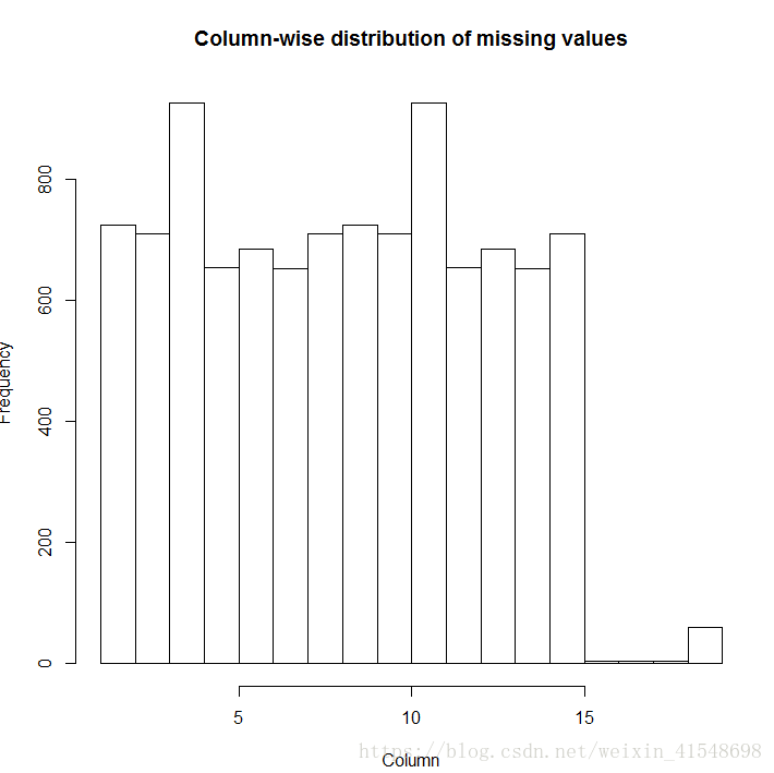
[1] "Missing Values: 10194"
[1] "Incomplete Records: 1377"
删除缺失值:
> nrow<-dim(dat)[1] # record the dimensions of the data (before removing anything!)
> dat<-na.omit(dat) # omit rows containing missing values
> nrow1<-dim(dat)[1] # record the new dimensions of the data (after removing NAs)
> removed(nrow, nrow1) # check how many records have been removed
[1] "number of records REMOVED: 1377"
[1] "number of records REMAINING: 51183"
计算能量发出和能量基准:
10分钟内发出的能量(KWH)、动能作为观察风速的函数、Betz限制、涡轮效率。
n<-length(dat$cum_energy_delivered_kwh)
a<-dat$cum_energy_delivered_kwh[1:n-1]
b<-dat$cum_energy_delivered_kwh[2:n]
diff<-b-a
dat$energy_sentout_10min_kwh<-c(diff,0)
风功率=(1/2)*RoO*面积*(速度)^=[kg/m^ 3 ] *[m^ 2 ] *[m/s] ^=[kg*m^ 2 /s^ 3 ]=[kg*m^ 2 /s^ 2 ] [1/s]=[牛顿米] / [第二]=[焦耳/秒]=[沃茨]
> rho=1.225
> area=2174
> turbines=7
> c <- (1/2)*rho*area
> dat$wind_power_kw <- c*(dat$mean_wind_mps)^3*turbines/1000
> dat$wind_energy_10min_kwh <- c*(dat$mean_wind_mps)^3*turbines/(1000*6)
> betz.coef <- 16/27
> dat$betz_limit_10min_kwh <- dat$wind_energy_10min_kwh*betz.coef
> dat$turbine_eff<-dat$energy_sentout_10min_kwh/dat$wind_energy_10min_kwh
> uncurtailed_power<-apply(X=dat[,2:8], MARGIN=1, FUN=sum)
> dat$uncurtailed_10min_kwh<-(uncurtailed_power)/6
> dat$curtailment_10min_kwh<-dat$uncurtailed-dat$energy_sentout_10min_kwh
检查是否有缺失值或异常值参与计算:
> check(dat)
[1] "Missing Values: 179"
[1] "Incomplete Records: 179"
删除缺失值:
> nan<-which(dat$turbine_eff == "NaN")
> dat$turbine_eff[nan]<-0
> inf<-which(dat$turbine_eff == "Inf")
> dat$turbine_eff[inf]<-0
>
> check(dat)
[1] "Missing Values: 0"
[1] "Incomplete Records: 0"
时间序列处理:
get<-which(is.na(as.POSIXlt(dat$date_time, format="%m/%d/%y %H:%M")))
dat$date_time[get]<-paste(dat$date_time[get], "00:00", sep=" ")
sum(is.na(as.POSIXlt(dat$date_time, format="%m/%d/%y %H:%M")))
dat$date_time<-as.POSIXlt(dat$date_time, format="%m/%d/%y %H:%M")
dat$month <- cut(dat$date_time, breaks = "month")
week <- cut(dat$date_time, breaks = "week")
day <- cut(dat$date_time, breaks = "day")
hour <- cut(dat$date_time, breaks = "hour")
dummy<-strsplit(as.character(week), split=" ")
week<-laply(dummy, '[[', 1) # keep the date, drop the time
dat$week<-as.factor(week)
dummy<-strsplit(as.character(day), split=" ")
day<-laply(dummy, '[[', 1) # keep the date, drop the time
dat$day<-as.factor(day)
dummy<-strsplit(as.character(hour), split=" ")
hour<-laply(dummy, '[[', 2) # keep the time, drop the date
dat$hour<-as.factor(hour)时间序列可视化:
energy<-subset(dat, select=c("day", "energy_sentout_10min_kwh", "wind_energy_10min_kwh", "betz_limit_10min_kwh", "uncurtailed_10min_kwh", "curtailment_10min_kwh"))
energy<-ddply(energy, .(day), numcolwise(sum))
test<-melt(energy, id.vars=("day"))
ggplot(test, aes(x=day, y=value/10^3, group=variable, colour=variable, linetype=variable)) +
geom_line() +
scale_y_continuous(name="MWh per day") +
labs(title="Energy Timeseries") +
theme_classic() +
scale_x_discrete(breaks=test$day[seq(1, 360, by=60)], labels=abbreviate)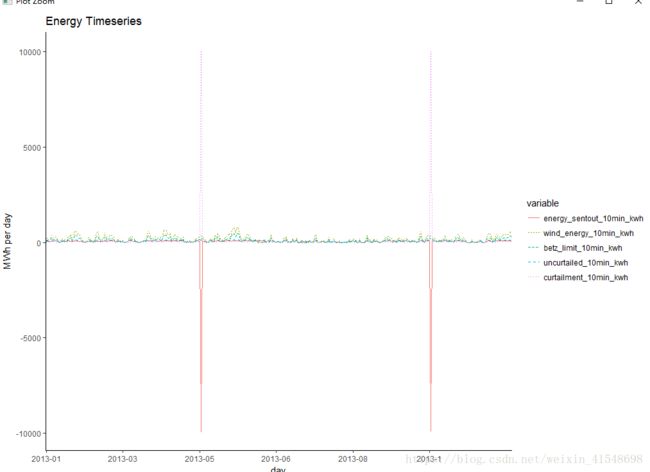
energy<-subset(dat, select=c("day","week", "month", "energy_sentout_10min_kwh", "wind_energy_10min_kwh", "betz_limit_10min_kwh", "uncurtailed_10min_kwh", "curtailment_10min_kwh"))
energy<-ddply(energy, .(day, week, month), numcolwise(sum))
test<-melt(energy, id.vars=c("day", "week", "month"))
levels(test$month) <- month.name[1:12]ggplot(test, aes(x=day, y=value/10^3, group=variable, colour=variable, linetype=variable)) +
geom_line() +
facet_wrap(~month, scales="free") +
scale_y_continuous(name="MWh per day") +
labs(title="Monthwise Energy Timeseries") +
theme_classic() +
scale_x_discrete(breaks=NULL)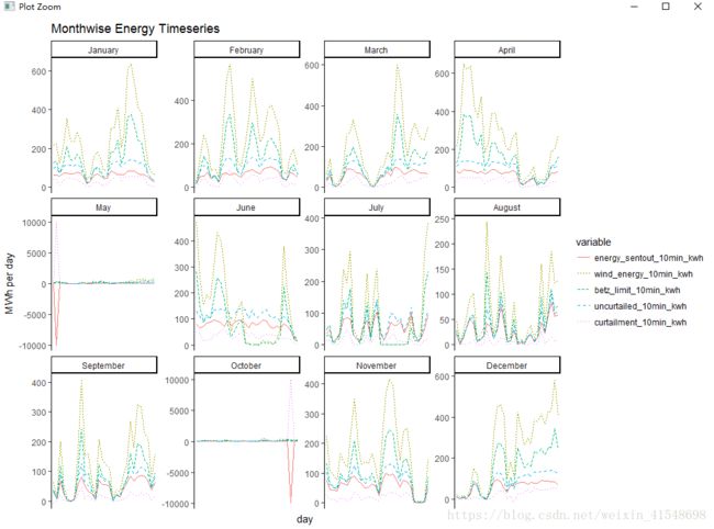
如图所示,有明显的异常值存在。
数据过滤器:
我们可以对发送的能量数据进行不同程度的筛选:
> summary(dat$energy_sentout_10min_kwh)
    Min.  1st Qu.   Median     Mean  3rd Qu.     Max.
-9999000      236      417       22      586    47120
hist(dat$energy_sentout_10min_kwh) 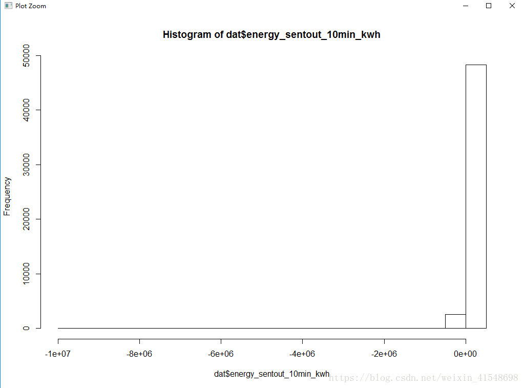
处理异常值:
> nrow<-dim(dat)[1]
> dat<-subset(dat, dat$energy_sentout_10min_kwh >= 0)
> nrow2<-dim(dat)[1]
> removed(nrow, nrow2)
[1] "number of records REMOVED: 2"
[1] "number of records REMAINING: 50824"
> capacity<-850*7 # 850 KW rated capacity x 7 turbines
> capacity_10min_kwh<-capacity*(10/60) # max energy sentout in 10 minutes
> dat<-subset(dat, dat$energy_sentout_10min_kwh <= capacity_10min_kwh)
> nrow3<-dim(dat)[1]
> removed(nrow2, nrow3)
[1] "number of records REMOVED: 39"
[1] "number of records REMAINING: 50785"
> summary(dat$energy_sentout_10min_kwh)
Min. 1st Qu. Median Mean 3rd Qu. Max.
0.0 235.0 417.0 411.6 585.0 964.0
> hist(dat$energy_sentout_10min_kwh)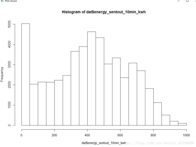
现在符合统计计算(正态分布)
看看数据在时间序列的可视化:
> energy<-subset(dat, select=c("week", "energy_sentout_10min_kwh", "uncurtailed_10min_kwh", "curtailment_10min_kwh", "betz_limit_10min_kwh"))
> energy<-ddply(energy, .(week), numcolwise(sum))
> test<-melt(energy, id.vars=("week"))
> ggplot(test, aes(x=week, y=value/10^3, group=variable, colour=variable, linetype=variable)) +
+     geom_line() +
+     scale_y_continuous(name="MWh per week") +
+     labs(title="Energy Timeseries") +
+     theme_classic() +
+     scale_x_discrete(breaks=levels(test$week)[seq(1,52, by=8)], labels=abbreviate)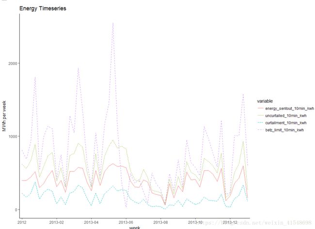
现在我们能够看到发送(缩减)的能量,可能的能量(未削减)和差异(缩减)的时间趋势。我们将Betz极限(理论最大值)作为基准比较。
使用风速的数据过滤器:
 summary(dat$mean_wind_mps)
   Min. 1st Qu.  Median    Mean 3rd Qu.    Max.
  0.000   5.700   8.600   8.116  10.900  18.800
> summary(dat$min_wind_mps)
   Min. 1st Qu.  Median    Mean 3rd Qu.    Max.
  0.000   3.700   6.000   5.625   7.800  15.800
> summary(dat$max_wind_mps)
   Min. 1st Qu.  Median    Mean 3rd Qu.    Max.
    0.0     7.7    11.1    10.6    13.9    31.5
> hist(dat$mean_wind_mps, main="Histogram of Mean Windspeeds")
> hist(dat$min_wind_mps, main="Histogram of Min Windspeeds")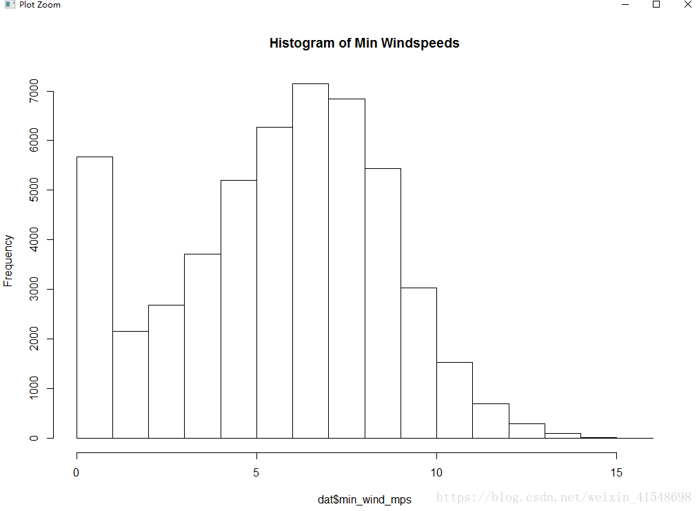
> hist(dat$max_wind_mps, main="Histogram of Max Windspeeds")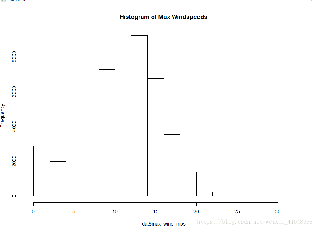
除了第一个仓外,风数据看起来还可以。第一个箱子太大了。所以我们删除了与风速低于0.5 mps(第一个仓)相关的记录(行)。
> dat<-subset(dat, mean_wind_mps > 0.5)根据时间检查分测量值:
wind<-subset(dat, select=c("week", "mean_wind_mps", "max_wind_mps", "min_wind_mps"))
wind<-ddply(wind, .(week), numcolwise(mean))

# plot wind vs time
test<-melt(wind, id.vars=("week"))
ggplot(test, aes(x=week, y=value, group=variable, colour=variable, linetype=variable)) +
  geom_line() +
  scale_y_continuous(name="Windspeed [m/s]") +
  labs(title="Wind Timeseries") +
  theme_classic() +
  scale_x_discrete(breaks=levels(test$week)[seq(1,360, by=30)], labels=abbreviate)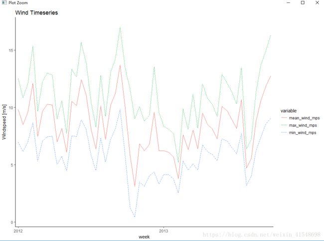
现在让我们来检查风速和能量测量是否合理(例如成对观测)。
回想一下这是时间序列数据,所以每个时间戳都有一个风速和能量测量。
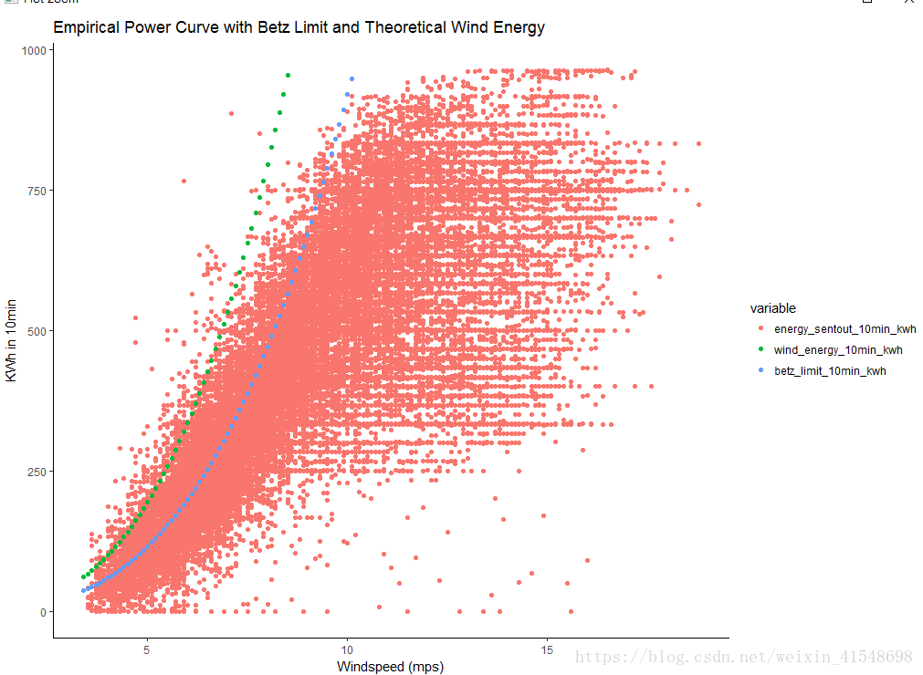
energy<-subset(dat, select=c("mean_wind_mps", "energy_sentout_10min_kwh", "wind_energy_10min_kwh", "betz_limit_10min_kwh"))
energy<-melt(energy, id.vars=("mean_wind_mps"))
ggplot(energy, aes(x=mean_wind_mps, y=value, group=variable, colour=variable)) +
  geom_point() +
  scale_y_continuous(name="KWh in 10min", limit=c(0, max(dat$energy_sentout_10min_kwh))) +
  scale_x_continuous(name="Windspeed (mps)") +
  labs(title="Empirical Power Curve with Betz Limit and Theoretical Wind Energy") +
  theme_classic()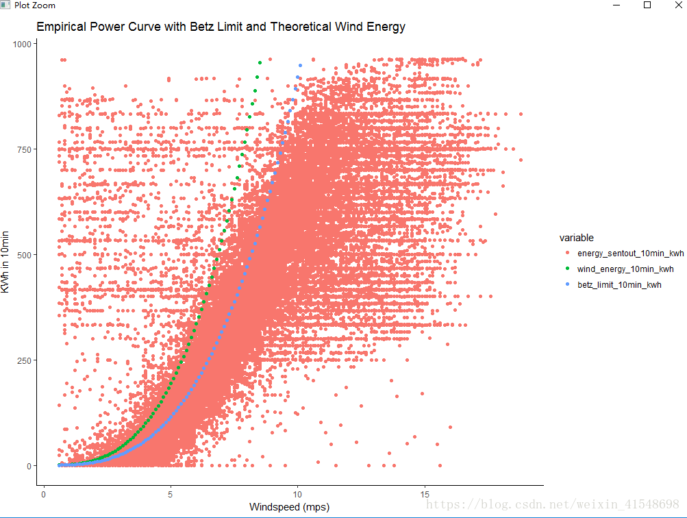
如果我们使用贝兹极限过滤数据,Windspeed vs功率输出看起来不错。否则,我们会看到贝兹极限以上的观测值,但我们知道这是不可能的。在如此低的风速下如何能够产生如此强大的动力呢?唯一的(可能的)解释是风的测量结果是关闭的。如果风压计(风速计)读数过低,则会人为地将点放在真实功率曲线的左侧,从而创建高于贝兹极限的点。在这里,我们能够应用物理系统的知识来改进数据过滤。
必要时我们可以添加更多的过滤器。
涡轮设定点
我们知道风机在风速低于3mps和25mps以上时停机。我们有两种选择来应用这些信息:选项1:删除所有风速<3 mps或> 25 mps的观测值。
* Pro:涡轮机已关闭,因此没有关于风速和发电之间关系的信息。
* Con:Weibull分布和容量因子将向上倾斜,因为低风速下的观测已被删除。
下面的代码没有运行,但作为如何根据涡轮机设定值过滤数据的示例显示。
保存“干净”的风力数据(后过滤器)
或者,我们可以使用此过滤器:选项2:当风速<3 mps或> 25 mps时,将功率设置为零(而不是完全按照选项1删除记录)。
* Pro:容量因子会更准确,因为我们在低风速下保留了观测值。* Con:拟合Weibull分布比较困难,因为大量的风速观测值被迫为零,从而形成了人为的较低的尾部。
filter<-which(dat$mean_wind_mps < 3 | dat$mean_wind_mps > 25)
dat$energy_sentout_10min_kwh[filter]<-0
将威布尔分布拟合到风速数据中
> library(fitdistrplus)
载入需要的程辑包:MASS
载入需要的程辑包:survival
> descdist(dat$mean_wind_mps)
summary statistics
------
min:  3.4   max:  18.8
median:  9.5
mean:  9.504264
estimated sd:  2.706452
estimated skewness:  0.1788128
estimated kurtosis: 2.493191 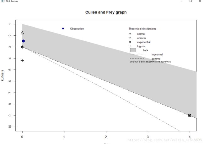
> weibull.fit<-fitdist(dat$mean_wind_mps, distr="weibull")
> summary(weibull.fit)
Fitting of the distribution ' weibull ' by maximum likelihood
Parameters :
       estimate Std. Error
shape  3.866578 0.01480657
scale 10.510752 0.01430917
Loglikelihood:  -97177.88   AIC:  194359.8   BIC:  194377
Correlation matrix:
          shape     scale
shape 1.0000000 0.3221711
scale 0.3221711 1.0000000

> plot(weibull.fit, demp=TRUE)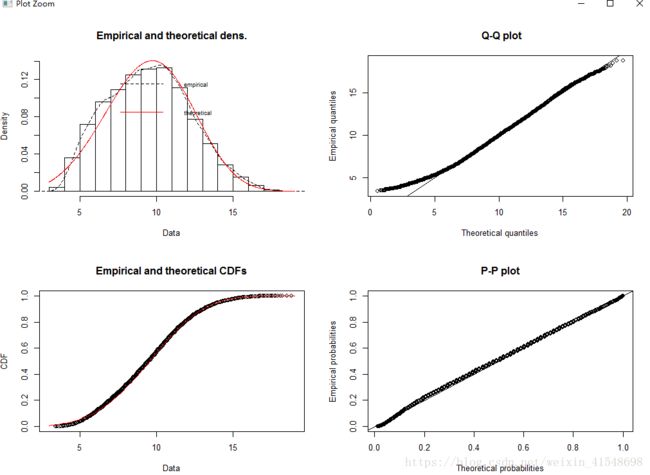
计算容量因子(实际和潜在)
> avg.power<-sum(dat$energy_sentout_10min_kwh)/(dim(dat)[1]/6)
>
> # summation of energy sentout, divided by the number of hours*capacity, yields capacity factor.
> actual.cap.factor<-sum(dat$energy_sentout_10min_kwh)/(850*7*dim(dat)[1]/6)
> uncurtailed.cap.factor<-sum(dat$uncurtailed_10min_kwh)/(850*7*dim(dat)[1]/6)
> betz.cap.factor<-sum(dat$betz_limit_10min_kwh)/(850*7*dim(dat)[1]/6)
>
> # display the results
> data.frame(actual.cap.factor, uncurtailed.cap.factor, betz.cap.factor)
  actual.cap.factor uncurtailed.cap.factor
1         0.4621844              0.6484466
  betz.cap.factor
1       0.9941704
数据修正
上面我们演示了几种基于系统物理和已知系统约束来过滤数据的方法。这种类型的数据过滤非常适合移除随机丢失,错误或异常数据。但是,如果我们有理由相信风测量系统性太低,会发生什么呢?我们如何解决数据中的系统性偏见?一种方法是应用校正算法。
风速校正算法
假设发出的能量测量结果是正确的,并且所有的误差都包含在风速测量中。这可能是一个很好的假设,因为能源数据可以在电力系统的其他地方得到确认(例如在巴士线上,由公用事业或调度中心等)。现在,假设负载测量是正确的,那么我们可以退出产生这么大功率所需的最小风速。然后,我们重新将计算的最小风速分配给不可行的风速测量值。从概念上讲,我们正在通过将它们移到右侧(到功率曲线)来纠正不准确的风速测量值。
为了演示数据修正作为删除可疑数据的替代方法,我们从一开始就从原始数据开始:
现在,我们移除统计离群值,但并不适用于基于物理的过滤器(如贝兹极限,涡轮机的设定值,等...)。
> nrow<-dim(dat)[1] # number of complete records BEFORE filtering
>
> # select the numeric or integer class columns
> c<-sapply(dat, class) # class of each column
> colIndex<-which(c=="numeric" | c=="integer") # column index of numeric or integer vectors
>
> # compute column-wise quantiles
> # apply(dat[,-1], 2, stats::quantile)
> range<-apply(dat[,colIndex], 2, function(x) {quantile(x, probs=c(.01, .99)) } )
>
> # get names of the columns that we want to filter on (all but the first column)
> # names<-colnames(dat[,colIndex])
> names<-names(colIndex) # identical to above
>
> # iterate through each column, subsetting the ENTIRE DATA.FRAME by removing records (rows) associated with an outlier value in that column
> for(i in 1:dim(range)[2]){
+     n<-dim(dat)[1] # number of rows at start
+     dat<-subset(dat, eval(parse(text=names[i])) > range[1,i])  # keep records above 1st percentile
+     dat<-subset(dat, eval(parse(text=names[i])) < range[2,i])  # keep records less than 99 percentile
+     p<-dim(dat)[1] # number of rows at end
+     print(paste(n-p, "records dropped when filtering:", toupper(names[i]), sep=" "))
+ }
[1] "1411 records dropped when filtering: T1_POSSIBLE_POWER"
[1] "574 records dropped when filtering: T2_POSSIBLE_POWER"
[1] "655 records dropped when filtering: T3_POSSIBLE_POWER"
[1] "1365 records dropped when filtering: T4_POSSIBLE_POWER"
[1] "567 records dropped when filtering: T5_POSSIBLE_POWER"
[1] "209 records dropped when filtering: T6_POSSIBLE_POWER"
[1] "342 records dropped when filtering: T7_POSSIBLE_POWER"
[1] "652 records dropped when filtering: T1_TOTAL_ACTIVE_POWER"
[1] "0 records dropped when filtering: T2_TOTAL_ACTIVE_POWER"
[1] "0 records dropped when filtering: T3_TOTAL_ACTIVE_POWER"
[1] "0 records dropped when filtering: T4_TOTAL_ACTIVE_POWER"
[1] "0 records dropped when filtering: T5_TOTAL_ACTIVE_POWER"
[1] "0 records dropped when filtering: T6_TOTAL_ACTIVE_POWER"
[1] "0 records dropped when filtering: T7_TOTAL_ACTIVE_POWER"
[1] "148 records dropped when filtering: MEAN_WIND_MPS"
[1] "348 records dropped when filtering: MIN_WIND_MPS"
[1] "101 records dropped when filtering: MAX_WIND_MPS"
[1] "726 records dropped when filtering: CUM_ENERGY_DELIVERED_KWH"
[1] "186 records dropped when filtering: ENERGY_SENTOUT_10MIN_KWH"
[1] "0 records dropped when filtering: WIND_POWER_KW"
[1] "0 records dropped when filtering: WIND_ENERGY_10MIN_KWH"
[1] "0 records dropped when filtering: BETZ_LIMIT_10MIN_KWH"
[1] "368 records dropped when filtering: TURBINE_EFF"
[1] "0 records dropped when filtering: UNCURTAILED_10MIN_KWH"
[1] "466 records dropped when filtering: CURTAILMENT_10MIN_KWH"
> nrow2<-dim(dat)[1]
> removed(nrow, nrow2)
[1] "number of records REMOVED: 8118"
[1] "number of records REMAINING: 32151"将威布尔分布拟合到统计过滤的风速数据上
> library(fitdistrplus)
> descdist(dat$mean_wind_mps)
summary statistics
------
min:  4.4   max:  15.8
median:  9.2
mean:  9.10786
estimated sd:  2.18531
estimated skewness:  0.02845082
estimated kurtosis: 2.277846 
> weibull.fit.2<-fitdist(dat$mean_wind_mps, distr="weibull")
> summary(weibull.fit.2)
Fitting of the distribution ' weibull ' by maximum likelihood
Parameters :
      estimate Std. Error
shape 4.676529 0.02025770
scale 9.964618 0.01254753
Loglikelihood:  -70722.76   AIC:  141449.5   BIC:  141466.3
Correlation matrix:
          shape     scale
shape 1.0000000 0.3206738
scale 0.3206738 1.0000000

> plot(weibull.fit.2, demp=TRUE)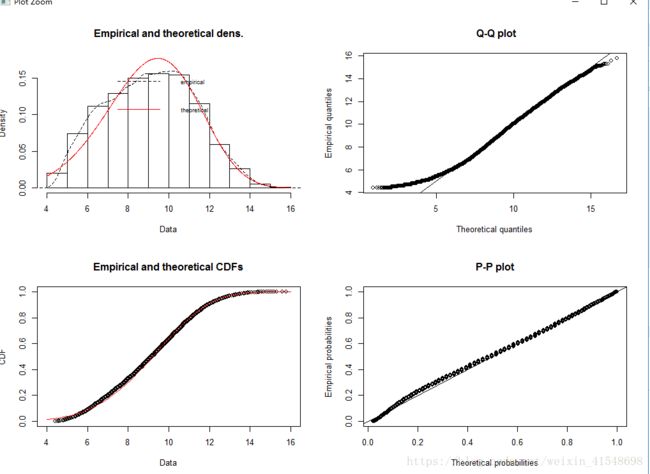
绘制风速与发电(缩减和未削减)
> plot(dat$mean_wind_mps, dat$uncurtailed_10min_kwh, col="red", cex=0.2, pch=20, main="Curtailed and Uncurtailed Wind Energy Production\nSao Vicente, Cape Verde (2013)", xlab="Windspeed (mps)", ylab="Energy (kWh/10min)")
> points(dat$mean_wind_mps, dat$energy_sentout_10min_kwh, col="green", cex=0.2, pch=20)
> legend("topleft", legend=c("Energy Possible (Uncurtailed)", "Energy Sentout (Curtailed)"), col=c("red", "green"), pch=20)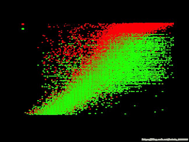
以下是我们的算法:对于每次观测,提供发出的能量(kWh),在功率曲线(kW)上找到最接近的匹配值,从功率曲线(mps)查询相应的风速。这成为修正的风速。只要测得的风速小于功率曲线指定的风速,就应用此功能。这将所有点移到功率曲线的左边,在右边。
代码是:
MPC<-read.table(file="v52-850KW-power-curve.csv", header=TRUE, strip.white=TRUE, sep=",")
MPC$design_sentout_10min_kwh<-MPC$power_kW*7/6 # kW x (7 turbines) x (1/6 hour)
MPC<-subset(MPC, windspeed_mps<25)

# plot the manufacturers power curve
plot(x=MPC$windspeed_mps, y=MPC$design_sentout_10min_kwh, type="p", pch=4, main="Manufacturers Power Curve\n with Empirical Overlay", xlab="Windspeed (mps)", ylab="Energy (kWh/10min)", xlim=range(dat$mean_wind_mps))
points(y=dat$energy_sentout_10min_kwh, x=dat$mean_wind_mps, col="green", cex=0.1, pch=20)
points(y=dat$uncurtailed_10min_kwh, x=dat$mean_wind_mps, col="red", cex=0.1, pch=20)
legend("bottomright", col=c("black", "green", "red"), pch=c(4, 20, 20), legend=c("Manufacturers Power Curve", "Energy Sentout (Curtailed)","Energy Possible (Uncurtailed)") )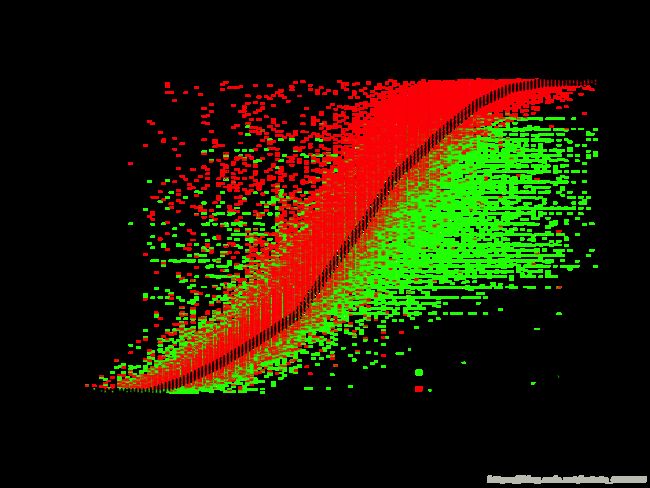
预测
拟合一个局部多项式功率曲线模型
现在我们已经描述了该区域的风速(威布尔分布),并估计了功率曲线(给定风速下的功率输出),我们可以从威布尔分布中抽样,生成新的风力数据并计算预期的功率输出。为了使功率曲线成为连续函数(而不是离散),我们拟合了一个多项式函数。本地多项式估计技术(例如,k最近的neigbor和核密度)为全球拟合提供了优势。在局部估计技术中,拟合是在小的邻域内进行的,从而以较低的多项式阶数提高拟合的良好性。这个概念类似于移动平均,并且平滑样条。这里我们拟合了两个局部多项式模型,一个用于观察,另一个用于制造商功率曲线。选择一个或另一个是一个偏好和理念问题(您是否相信涡轮机能够精确符合制造商的技术规格,或者您是否相信自己的测量?)
library(locfit)
empirical.mod<-locfit(energy_sentout_10min_kwh ~ mean_wind_mps, data=dat)
summary(empirical.mod)
## Estimation type: Local Regression
##
## Call:
## locfit(formula = energy_sentout_10min_kwh ~ mean_wind_mps, data = dat)
##
## Number of data points: 36413
## Independent variables: mean_wind_mps
## Evaluation structure: Rectangular Tree
## Number of evaluation points: 7
## Degree of fit: 2
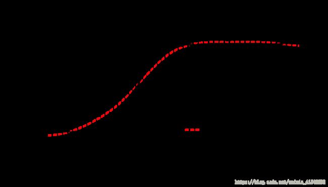
## Fitted Degrees of Freedom: 5.29plot(empirical.mod, main="Model Fit to Empirical Data")
points(y=dat$energy_sentout_10min_kwh, x=dat$mean_wind_mps, cex=0.1, pch=20, col="red")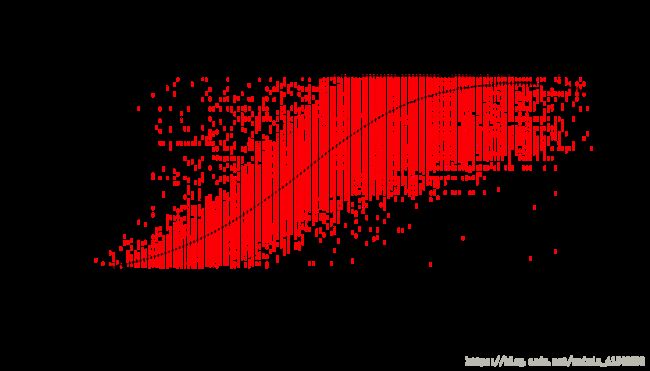
manufacturer.mod<-locfit(design_sentout_10min_kwh ~ windspeed_mps, data=MPC)
summary(manufacturer.mod)
## Estimation type: Local Regression
##
## Call:
## locfit(formula = design_sentout_10min_kwh ~ windspeed_mps, data = MPC)
##
## Number of data points: 560
## Independent variables: windspeed_mps
## Evaluation structure: Rectangular Tree
## Number of evaluation points: 5
## Degree of fit: 2
## Fitted Degrees of Freedom: 4.822plot(manufacturer.mod, lty=2, col="red", main="Model Fit to Manufacturers Power Curve", lwd=1)
lines(y=MPC$design_sentout_10min_kwh, x=MPC$windspeed_mps, col="black", lty=1, lwd=1)
legend("bottomright", legend=c("Manufacturer's Power Curve", "Local Polynomial Model Fit"), col=c("black", "red"), lty=c(1,2), lwd=c(1, 1))
预测模型
现在我们可以根据风速的概率(威布尔)分布和拟合功率曲线模型(局部多项式)来预测能量产生。
expected.wind=rweibull(8760*6, shape=weibull.fit$estimate[1], scale=weibull.fit$estimate[2])
# estimate generation given expected windspeeds
expected.gen.empirical<-predict(empirical.mod, newdata=expected.wind)
expected.gen.manufacturer<-predict(manufacturer.mod, newdata=expected.wind)
# calculate the expected (uncurtailed) capacity factor for next year:
sum(expected.gen.empirical)/(850*7*8760)
## [1] 0.3902
sum(expected.gen.manufacturer)/(850*7*8760)
## [1] 0.4949
# plot the new (expected) power curve
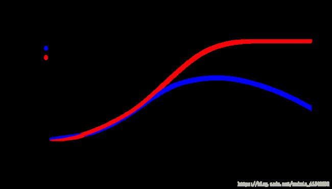
plot(expected.gen.empirical ~ expected.wind, col="blue", ylim=c(0, 850*7/6), xlim=c(0,20), pch=20, main="Comparing Two Prediction Techniques", ylab="Expected Gen. (kWh/10min)", xlab="Expected Wind (mps)")
points(y=expected.gen.manufacturer, x=expected.wind, col="red", pch=20)
legend("topleft", legend=c("Fit to Empirical Data", "Fit to Manufacturer's Power Curve"), col=c("blue", "red"), pch=c(20,20))