Log-Linear Model & CRF 条件随机场详解

往期文章链接目录

Log-Linear model

Let $x$ be an example, and let $y$ be a possible label for it. A log-linear model assumes that

$$p(y|x;w)=\frac{\exp [{\sum }_{j=1}^J{w}_j{F}_j(x,y)]}{Z(x,w)}$$

where the partition function

$$Z(x,w)=\sum _{y^{\prime }}\exp [\sum _{j=1}^J{w}_j{F}_j\left(x,y^{\prime }\right)]$$

Note that in ${\sum }_{y^{\prime }}$, we make a summation over all possible $y$. Therefore, given $x$, the label predicted by the model is

$$\hat{y}=\underset{y}{\mathrm{argmax}}p(y|x;w)=\underset{y}{\mathrm{argmax}}\sum _{j=1}^J{w}_j{F}_j(x,y)$$

Each expression $F_j(x,y)$ is called a feature-function. You can think of it as the $j$-th feature extracted from $(x,y)$.

Remark of the log-linear model:

• a linear combination ${\sum }_{j=1}^J{w}_j{F}_j(x,y)$ can take any positive or negative real value; the exponential makes it positive.

• The division makes the result $p(y|x;w)$ between 0 and 1, i.e. makes them be valid probabilities.

Conditional Random Fields (CRF)

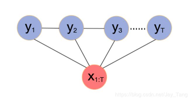
Last time, we talked about Markov Random Fields. In this post, we are going to discuss Conditional Random Fields, which is an important special case of Markov Random Fields arises when they are applied to model a conditional probability distribution $p(y|x)$, where $x$ and $y$ are vactor-valued variables.

Formal definition of CRF

Formally, a CRF is a Markov network which specifies a conditional distribution

$$P(y\mid x)=\frac{1}{Z(x)}\prod _{c\in C}{\varphi }_c(x_c,y_c)$$

with partition function

$$Z=\sum _{y\in \mathcal{Y}}\prod _{c\in C}{\varphi }_c(x_c,y_c)$$

we further assume that the factors ${\varphi }_c(x_c,y_c)$ (maximal cliques) are of the form

$${\varphi }_c(x_c,y_c)=\exp [w_c^T{f}_c(x_c,y_c)]$$

Since we require our potential function $\varphi$ to be non-negative, it’s natural to use the exponential function. $f_c(x_c,y_c)$ can be an arbitrary set of features describing the compatibility between $x_c$ and $y_c$. Note that these feature functions could be designed by manually doing feature engineering or using deep learning, LSTM, etc.

Log-linear model to linear-CRF

As a remainder, let $x$ be an example, and let $y$ be a possible label for it. Then a log-linear model assumes that

$$p(y|x;w)=\frac{\exp [{\sum }_{j=1}^J{w}_j{F}_j(x,y)]}{Z(x,w)}$$

From now on, we use the bar notation for sequences. Then to linear-CRF, we write the above equation as

$$\begin{array}{rlrl}p(\bar{y}|\bar{x};w)& =\frac{\exp [{\sum }_{j=1}^J{w}_j{F}_j(\bar{x},\bar{y})]}{Z(\bar{x},w)}& & \\ & =\frac{\exp [{\sum }_{j=1}^J{w}_j{\sum }_{i=2}^T{f}_j(y_{i-1},y_i,\bar{x})]}{Z(\bar{x},w)}& & (1)\end{array}$$

where $y$ can take values from $\{1,2,...,m\}$. Here is an example:

Assume we have a sequence $\bar{x}=(x_1,x_2,x_3,x_4)$ and the corresponding hidden sequence $\bar{y}=(y_1,y_2,y_3,y_4)$.

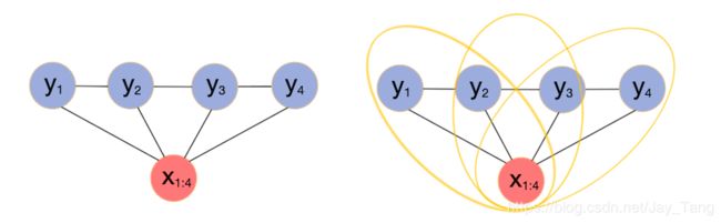
We can divide each feature-function $F_j(\bar{x},\bar{y})$ into fuctions for each maximal clique. That is,

$$F_j(\bar{x},\bar{y})=\sum _{i=2}^T{f}_j(y_{i-1},y_i,\bar{x})\text{\hspace{1em}(1.1)}$$

Perticularly, from the above figure, since we have $3$ maximal cliques, so

$$F_j(\bar{x},\bar{y})=f_j(y_1,y_2,\bar{x})+f_j(y_2,y_3,\bar{x})+f_j(y_3,y_4,\bar{x})$$

If we extract $J$ feature functions from the $(\bar{x},\bar{y})$ pair, then it becomes

$$\sum _{j=1}^J{w}_j{F}_j(x,y)=\sum _{j=1}^J{w}_j\sum _{i=2}^T{f}_j(y_{i-1},y_i,\bar{x})$$

Inference problem for CRF

• Goal: given a sequence $\bar{x}$, and parameter $w$, find the best hidden sequence $\bar{y}$. The condition probability of $\bar{y}$ is

$$p(\bar{y}|\bar{x};w)=\frac{\exp [{\sum }_{j=1}^J{w}_j{\sum }_{i=2}^T{f}_j(y_{i-1},y_i,\bar{x})]}{Z(\bar{x},w)}$$

Our objective is（check that the objective of CRF is the objective of Log-Linear model described above）:

$$\begin{array}{rlrl}\hat{y}& =\underset{\bar{y}}{\mathrm{argmax}}p(\bar{y}|\bar{x};w)& & (2)\\ & =\underset{\bar{y}}{\mathrm{argmax}}\sum _{j=1}^J{w}_j\sum _{i=2}^T{f}_j(y_{i-1},y_i,\bar{x})& & (3)\\ & =\underset{\bar{y}}{\mathrm{argmax}}\sum _{i=2}^T{g}_i(y_{i-1},y_i)& & (4)\end{array}$$

Note:

• $(2)\to (3)$: we can ignore the denominator since it stays the same for all possible $\bar{y}$. Exponential function won’t affect our objective.

• We set
  $$g_i(y_{i-1},y_i)=\sum _{j=1}^J{w}_j\cdot f_j(y_{i-1},y_i,\bar{x})\text{\hspace{1em}(5)}$$

Based on our objective in $(5)$, we want to find the best path from $y_1$ to $y_T$ such that the objective function is maximized. Clearly, we can use Dynamic Programming (DP) here.

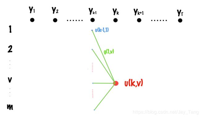
Let $u(k,v)$ denote the score of the best path from $t=1$ to $t=k$, where the tag of time $k$ is $v$. Then the recursion formula can be easily visualized from the above figure and we can write it as

$$u(k,v)=\underset{s}{\max }[u(k-1,s)+g_k(s,v)]$$

where $s$ takes values from states $\{1,2,...,m\}$. The maximum of the objective is $\max \{u(T,1),u(T,2),...,u(T,m)\}$.

• Time complexity: $O(mT)\cdot O(m)=O(m^{2}T)$.

• Space complexity: $O(mT)$ since we need to track the path of the best sequence $\bar{y}$.

Learning problem for CRF

Goal: Given the data set $D=\{(x^{(1)},y^{(1)}),...,(x^{(n)},y^{(n)})\}$, we want to find parameter $w$ to maximize $p(D|w)$. That is,

$$\begin{array}{rl}{\hat{w}}_{MLE}& =\underset{w}{\max }p(D|w)\\ & =\underset{w}{\max }\prod _{i=1}^{n}p(y^{(i)}|x^{(i)};w)\end{array}$$

That is, we need to take derivatives and then use the gradient descent method.

Learning problem for general Log-Linear model

$$p(\bar{y},\bar{x};w)=\frac{\exp [{\sum }_{j=1}^J{w}_j{F}_j(x,y)]}{Z(x,w)}$$

Take the derivative with respect to $w_j$:

$$\begin{array}{rlrl}\frac{\partial }{\partial w_j}[\log p(y|x;w)]& =\frac{\partial }{\partial w_j}[\sum _{j=1}^J{w}_j{F}_j(x,y)-\log Z(x,w)]& & \\ & =F_j(x,y)-\frac{1}{Z(x,w)}\cdot \frac{\partial }{\partial w_j}Z(x,w)& & (6)\end{array}$$

where

$$\begin{array}{rlrl}\frac{\partial }{\partial w_j}Z(x,w)& =\frac{\partial }{\partial w_j}\sum _{y^{\prime }}\exp [\sum _{j=1}^J{w}_j{F}_j\left(x,y^{\prime }\right)]& & \\ & =\sum _{y^{\prime }}\frac{\partial }{\partial w_j}[\exp \sum _{j=1}^J{w}_j{F}_j\left(x,y^{\prime }\right)]& & \\ & =\sum _{y^{\prime }}[\exp \sum _{j=1}^J{w}_j{F}_j\left(x,y^{\prime }\right)]\cdot F_j\left(x,y^{\prime }\right)& & (7)\end{array}$$

Combining $(6)$ and $(7)$, we have

$$\begin{array}{rlrl}\frac{\partial }{\partial w_j}[\log p(y|x;w)]& =F_j\left(x,y\right)-\frac{1}{Z(x,w)}\sum _{y^{\prime }}{F}_j\left(x,y^{\prime }\right)[\exp \sum _{j=1}^J{w}_j{F}_j\left(x,y^{\prime }\right)]& & \\ & =F_j\left(x,y\right)-\sum _{y^{\prime }}{F}_j\left(x,y^{\prime }\right)\frac{\exp {\sum }_{j=1}^J{w}_j{F}_j\left(x,y^{\prime }\right)}{Z(x,w)}& & \\ & =F_j\left(x,y\right)-\sum _{y^{\prime }}{F}_j\left(x,y^{\prime }\right)\cdot p(y^{\prime }|x;w)& & \\ & =F_j\left(x,y\right)-E_{y^{\prime }\sim p(y^{\prime }|x;w)}[F_j\left(x,y^{\prime }\right)]& & (8)\end{array}$$

Learning problem for CRF

We can edit $(8)$ to get the partial derivative for CRF:

$$\begin{array}{rlrl}\frac{\partial }{\partial w_j}[\log p(\bar{y}|\bar{x};w)]& =F_j\left(\bar{x},\bar{y}\right)-E_{{\bar{y}}^{\prime }\sim p({\bar{y}}^{\prime }|x;w)}[F_j\left(x,{\bar{y}}^{\prime }\right)]& & (9)\\ & =F_j\left(\bar{x},\bar{y}\right)-E_{{\bar{y}}^{\prime }}[\sum _{i=2}^T{f}_j(y_{i-1},y_i,\bar{x})]& & (10)\\ & =F_j\left(\bar{x},\bar{y}\right)-\sum _{i=2}^T{E}_{{\bar{y}}^{\prime }}[f_j(y_{i-1},y_i,\bar{x})]& & (11)\\ & =F_j\left(\bar{x},\bar{y}\right)-\sum _{i=2}^T{E}_{y_{i-1},y_i}[f_j(y_{i-1},y_i,\bar{x})]& & (12)\\ & =F_j\left(\bar{x},\bar{y}\right)-\sum _{i=2}^T\sum _{y_{i-1}}\sum _{y_i}{f}_j(y_{i-1},y_i,\bar{x})\cdot p(y_{i-1},y_i|\bar{x};w)& & (13)\end{array}$$

Note:

• $(9)\to (10)$: Use equation $(1)$.

• $(11)\to (12)$: each term $f_j(y_{i-1},y_i,\bar{x})$ is only related to $y_{i-1}$ and $y_i$.

• In the equation $(13)$, the only unknown term is $p(y_{i-1},y_i|\bar{x};w)$. Let’s now see how to compute it.

Compute $Z(\bar{x},w)$

$$\begin{array}{rlrl}Z(\bar{x},w)& =\sum _{\bar{y}}\exp \left[\sum _{j=1}^J{w}_j{F}_j\left(\bar{x},\bar{y}\right)\right]& & \\ & =\sum _{\bar{y}}\exp \left[\sum _{j=1}^J{w}_j\sum _{i=2}^T{f}_j(y_{i-1},y_i,\bar{x})\right]& & \\ & =\sum _{\bar{y}}\left[\exp \sum _{i=2}^T{g}_i(y_{i-1},y_i)\right]& & (14)\end{array}$$

We see the term $g_i(y_{i-1},y_i)$ in the equation $(14)$ again, and $(14)$ is the sum of $\left[\exp {\sum }_{i=2}^T{g}_i(y_{i-1},y_i)\right]$ over all $y$. If we list all the possibilities, the time complexity is $O(m^T)$, which is not acceptable. So we should solve it in a similar way like what we did in the inference section (Dynamic Programming). There are two ways to solve it: forward algorithm and backward algorithm. Note that this is very similar to HMM we discussed before.

Forward Algorithm

Let $\alpha (k,v)$ denote the sum of all possible paths from $t=1$ to $t=k$, where the tag of time $k$ is $v$. Then the recursion formula can be easily visualized from the above figure and we can write it as

$$\alpha (k,v)=\underset{s}{\max }\left[\alpha (k-1,s)\cdot \text{exp}{g}_k(s,v)\right]$$

where $s\in \{1,2,...,m\}$. Then, we can write $Z(\bar{x},w)$ as

$$Z(\bar{x},w)=\sum _{s=1}^m\alpha (T,s)$$

Backward Algorithm

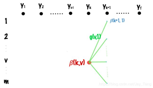
Let $\beta (k,v)$ denote the sum of all possible paths from $t=k$ to $t=T$, where the tag of time $t$ is $v$. Then the recursion formula can be easily visualized from the above figure and we can write it as

$$\beta (k,v)=\underset{s}{\max }\left[\beta (k+1,s)\cdot \text{exp}{g}_{k+1}(v,s)\right]$$

where $s\in \{1,2,...,m\}$. Then, we can write $Z(\bar{x},w)$ as

$$Z(\bar{x},w)=\sum _{s=1}^m\beta (1,s)$$

Compute $p(y_k=u|\bar{x};w)$

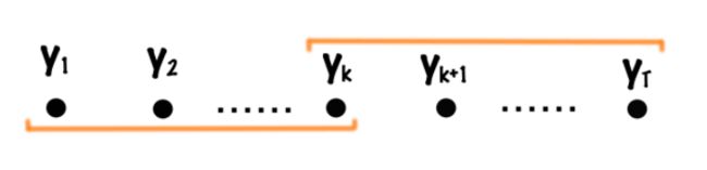
From the figure above, we can divide it into the product of a forward term and a backward term:

$$p(y_k=u|\bar{x};w)=\frac{\alpha (k,u)\cdot \beta (k,u)}{Z(\bar{x},w)}$$

where

$$Z(\bar{x},w)=\sum _u\alpha (k,u)\cdot \beta (k,u)$$

• Note that we can also compute $Z(\bar{x},w)$ by write it as a product of an $\alpha$ term and a $\beta$ term.

Compute $p(y_k=u,y_{k+1}=v|\bar{x};w)$

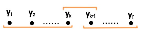
From the figure above, we can divide it into the product of a forward term, a backward term, and an term that represent the path going from $y_k=u$ to $y_{k+1}=v$:

$$p(y_k=u,y_{k+1}=v|\bar{x};w)=\frac{\alpha (k,u)\cdot [\text{exp}{g}_{k+1}(u,v)]\cdot \beta (k+1,v)}{Z(\bar{x},w)}$$

where

$$Z(\bar{x},w)=\sum _u\sum _v\alpha (k,u)\cdot [\text{exp}{g}_{k+1}(u,v)]\cdot \beta (k+1,v)$$

Now go back to where we stopped (equation $(13)$), and use what we just derived above, we have

$$\begin{array}{rlrl}\frac{\partial }{\partial w_j}[\log p(\bar{y}|\bar{x};w)]& =F_j\left(\bar{x},\bar{y}\right)-\sum _{i=2}^T\sum _{y_{i-1}}\sum _{y_i}{f}_j(y_{i-1},y_i,\bar{x})\cdot p(y_{i-1},y_i|\bar{x};w)& & \\ & =F_j\left(\bar{x},\bar{y}\right)-\sum _{i=2}^T\sum _{y_{i-1}}\sum _{y_i}{f}_j(y_{i-1},y_i,\bar{x})\cdot \frac{\alpha (i-1,y_{i-1})\cdot [\text{exp}{g}_i(y_{i-1},y_i)]\cdot \beta (i,y_1)}{Z(\bar{x},w)}& & (15)\end{array}$$

Now every term in the equation $(15)$ is known. So we can use SGD to update the parameter $w$.

---

Reference:

• https://ermongroup.github.io/cs228-notes/representation/undirected/
• http://cseweb.ucsd.edu/~elkan/250B/CRFs.pdf
• http://homepages.inf.ed.ac.uk/csutton/publications/crftut-fnt.pdf
• http://cseweb.ucsd.edu/~elkan/250Bfall2007/loglinear.pdf

往期文章链接目录