08_Dimensionality Reduction_svd_Kernel_pca_make_swiss_roll_subplot2grid_IncrementalPCA_memmap_LLE
cp5_Compressing Data via Dimensionality Reduction_feature extraction_PCA_LDA_convergence_kernel PCA:
https://blog.csdn.net/Linli522362242/article/details/105196037
Reduction_svd( (singular values)^2 ==eigenvalues)
Many Machine Learning problems involve thousands or even millions of features for each training instance. Not only does this make training extremely slow, it can also make it much harder to find a good solution, as we will see. This problem is often referred to as the curse of dimensionality维度诅咒.
Fortunately, in real-world problems, it is often possible to reduce the number of features considerably, turning an intractable难对付的 problem into a tractable易处理的 one. For example, consider the MNIST images (introduced in
https://blog.csdn.net/Linli522362242/article/details/103786116): the pixels on the image borders are almost always white, so you could completely drop these pixels from the training set without losing much information. Figure 7-6 confirms that these pixels are utterly完全地 unimportant for the classification task. Moreover, two neighboring pixels are often highly correlated: if you merge them into a single pixel (e.g., by taking the mean of the two pixel intensities), you will not lose much information.
############################################
WARNING
Reducing dimensionality does lose some information (just like compressing an image to JPEG can degrade its quality), so even though it will speed up training, it may also make your system perform slightly worse. It also makes your pipelines a bit more complex and thus harder to maintain. So you should first try to train your system with the original data before considering using dimensionality reduction if training is too slow. In some cases, however, reducing the dimensionality of the training data may filter out some noise and unnecessary details and thus result in higher performance (but in general it won't; it will just speed up training).
############################################
Apart from speeding up training, dimensionality reduction is also extremely useful for data visualization (or DataViz). Reducing the number of dimensions down to two (or three) makes it possible to plot a high dimensional training set on a graph and often gain some important insights by visually detecting patterns, such as clusters.
we will discuss the curse of dimensionality and get a sense of what goes on in high dimensional space. Then, we will present the two main approaches to dimensionality reduction (projection and Manifold Learning流形学习), and we will go through three of the most popular dimensionality reduction techniques: PCA主成分分析, Kernel PCA核主成分分析, and LLE局部线性嵌入.
The Curse of Dimensionality
We are so used to living in three dimensions that our intuition fails us when we try to imagine a high dimensional space. Even a basic 4D hypercube is incredibly令人难以置信的 hard to picture in our mind (see Figure 8-1), let alone a 200 dimensional ellipsoid bent in a 1,000-dimensional space.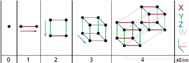
Figure 8-1. Point, segment, square, cube, and tesseract (0D to 4D hypercubes)
It turns out that many things behave very differently in high-dimensional space. For example, if you pick a random point in a unit square (a 1 × 1 square), it will have only about a 0.4% chance of being located less than 0.001 from a border(1-0.998^2=0.003996=0.4%, horizontal probability not in that range(0.001)=0.998, vertical probability not in that range=0.998, so the probability in 2D not in that range = 0.998^2) (in other words, it is very unlikely that a random point will be “extreme” along any dimension). But in a 10,000-dimensional unit hypercube (a 1 × 1 × ...× 1 cube, with ten thousand 1s), this probability is greater than 99.999999%(=1-0.998^10000). Most points in a high-dimensional hypercube are very close to the border.
Here is a more troublesome difference: if you pick two points randomly in a unit square, the distance between these two points will be, on average, roughly 0.52. If you pick two random points in a unit 3D cube, the average distance will be roughly 0.66. But what about two points picked randomly in a 1,000,000-dimensional hypercube? Well, the average distance, believe it or not, will be about 408.25 (roughly ![]() This is quite counterintuitive: how can two points be so far apart when they both lie within the same unit hypercube? This fact implies that highdimensional datasets are at risk of being very sparse: most training instances are likely to be far away from each other. Of course, this also means that a new instance will likely be far away from any training instance, making predictions much less reliable than in lower dimensions, since they will be based on much larger extrapolations推断. In short, the more dimensions the training set has, the greater the risk of overfitting it.
This is quite counterintuitive: how can two points be so far apart when they both lie within the same unit hypercube? This fact implies that highdimensional datasets are at risk of being very sparse: most training instances are likely to be far away from each other. Of course, this also means that a new instance will likely be far away from any training instance, making predictions much less reliable than in lower dimensions, since they will be based on much larger extrapolations推断. In short, the more dimensions the training set has, the greater the risk of overfitting it.
In theory, one solution to the curse of dimensionality could be to increase the size of the training set to reach a sufficient density of training instances. Unfortunately, in practice, the number of training instances required to reach a given density grows exponentially with the number of dimensions. With just 100 features (much less than in the MNIST problem), you would need more training instances than atoms in the observable universe in order for training instances to be within 0.1 of each other on average, assuming they were spread out uniformly across all dimensions.
Main Approaches for Dimensionality Reduction
Before we dive into specific dimensionality reduction algorithms, let's take a look at the two main approaches to reducing dimensionality: projection and Manifold Learning流形学习.
Projection
In most real-world problems, training instances are not spread out uniformly均匀分布 across all dimensions. Many features are almost constant, while others are highly correlated (as discussed earlier for MNIST). As a result, all training instances actually lie within (or close to) a much lower-dimensional subspace of the high-dimensional space. This sounds very abstract, so let’s look at an example. In Figure 8-2 you can see a 3D dataset represented by the circles.

Figure 8-2. A 3D dataset lying close to a 2D subspace一个3D数据集坐落在接近于2D子空间
from matplotlib.patches import FancyArrowPatch
from mpl_toolkits.mplot3d import proj3d

class Arrow3D( FancyArrowPatch ):
    def __init__(self, xs, ys, zs, *args, **kwargs):
                                  #arrow tail  #head  #tuple #dict
                                        #posA  #posB
        FancyArrowPatch.__init__(self, (0,0), (0,0), *args, **kwargs)
        self.verts3d = xs, ys, zs

    def draw(self, renderer):
        xs3d, ys3d, zs3d = self.verts3d
        xs, ys, zs = proj3d.proj_transform( xs3d, ys3d, zs3d, renderer.M )
                             #posA         #posB
        self.set_positions( (xs[0],ys[0]), (xs[1],ys[1]) )
        FancyArrowPatch.draw( self, renderer )


# Express the plane as a function of x and y

from sklearn.decomposition import PCA
import numpy as np

np.random.seed(4)
m=60
w1, w2 = 0.1, 0.3
noise = 0.1

angles = np.random.rand(m) * 3 * np.pi/2 -0.5
X = np.empty((m,3)) # (number of instance, 3 dimensions)
X[:,0] = np.cos(angles) + np.sin(angles)/2 + noise*np.random.randn(m)/2
X[:,1] = np.sin(angles)*0.7 + noise*np.random.randn(m)/2
X[:,2] = X[:,0]*w1 + X[:,1]*w2 + noise*np.random.randn(m)

pca = PCA( n_components=2 )
X2D = pca.fit_transform(X)
X3D_inv = pca.inverse_transform(X2D)

axes=[-1.8,1.8, -1.3,1.3, -1.0,1.0]

x1s = np.linspace(axes[0], axes[1], 10)
x2s = np.linspace(axes[2], axes[3], 10)
x1,x2 = np.meshgrid(x1s, x2s)

#pca.components_
#array([[-0.93636116, -0.29854881, -0.18465208],
#       [ 0.34027485, -0.90119108, -0.2684542 ]])
C = pca.components_
R = C.T.dot(C) # shape(3,2)xshape(2,3) => shape(3,3)
z = ( R[0,2]*x1 + R[1,2]*x2 ) / (1-R[2,2] )


# Plot the 3D dataset, the plane and the projections on that plane.
from mpl_toolkits.mplot3d import Axes3D
import matplotlib.pyplot as plt

fig = plt.figure( figsize=(12,7.6) )
ax = fig.add_subplot(111, projection='3d')

X3D_above = X[ X[:,2]>X3D_inv[:,2] ]
X3D_below = X[ X[:,2]<=X3D_inv[:,2] ]

# original point
ax.plot( X3D_below[:,0], X3D_below[:,1], X3D_below[:,2], "bo" ) #, alpha=0.5
ax.plot( X3D_above[:, 0], X3D_above[:,1], X3D_above[:,2], "yo" )
# inverse point
ax.plot( X3D_inv[:,0], X3D_inv[:,1], X3D_inv[:,2], "k+" )
ax.plot( X3D_inv[:,0], X3D_inv[:,1], X3D_inv[:,2], "k." )

ax.plot_surface(x1,x2,z, alpha=0.2, color="k")
np.linalg.norm(C, axis=0) #default l2: array([0.99627265, 0.94935597, 0.32582825])
ax.add_artist( Arrow3D( [0, C[0,0]], [0,C[0,1]], [0,C[0,2]], mutation_scale=15,
                       lw=1, arrowstyle="-|>", color="k")
             ) #C[0,:] is first component
ax.add_artist( Arrow3D( [0, C[1,0]], [0,C[1,1]], [0,C[1,2]], mutation_scale=15,
                       lw=1, arrowstyle="-|>", color="k")
             ) #C[1,:] is second component

for i in range(m): # m=60 instances
    if X[i,2] > X3D_inv[i,2]:
        ax.plot( [X[i][0], X3D_inv[i][0]], [X[i][1], X3D_inv[i][1]], [X[i][2], X3D_inv[i][2]], "k-" )
    else:
        ax.plot( [X[i][0], X3D_inv[i][0]], [X[i][1], X3D_inv[i][1]], [X[i][2], X3D_inv[i][2]], "k-",
                #color="#505050"
               )

ax.set_xlabel( "$x_1$", fontsize=18, labelpad=10 )
ax.set_ylabel( "$x_2$", fontsize=18, labelpad=10 )
ax.set_zlabel( "$x_3$", fontsize=18, labelpad=10 )
# axes=[-1.8,1.8, -1.3,1.3, -1.0,1.0]
ax.set_xlim( axes[0:2] )
ax.set_ylim( axes[2:4] )
ax.set_zlim( axes[4:6] )

plt.show()   #see previously right-figure
Notice that all training instances lie close to a plane: this is a lower-dimensional (2D) subspace of the high-dimensional (3D) space. Now if we project every training instance perpendicularly onto this subspace (as represented by the short lines connecting the instances to the plane), we get the new 2D dataset shown in Figure 8-3. Ta-da! We have just reduced the dataset’s dimensionality from 3D to 2D. Note that the axes correspond to new features z1 and z2 (the coordinates of the projections on the plane).

Figure 8-3. The new 2D dataset after projection
from sklearn.decomposition import PCA
import matplotlib.pyplot as plt
import numpy as np

np.random.seed(4)
m=60
w1, w2 = 0.1, 0.3
noise = 0.1

angles = np.random.rand(m) * 3 * np.pi/2 -0.5
X = np.empty((m,3)) # (number of instance, 3 dimensions)
X[:,0] = np.cos(angles) + np.sin(angles)/2 + noise*np.random.randn(m)/2
X[:,1] = np.sin(angles)*0.7 + noise*np.random.randn(m)/2
X[:,2] = X[:,0]*w1 + X[:,1]*w2 + noise*np.random.randn(m)

pca = PCA( n_components=2 )
X2D = pca.fit_transform(X)
X3D_inv = pca.inverse_transform(X2D)

fig = plt.figure()
ax = fig.add_subplot(111, aspect="equal")

ax.plot(X2D[:,0], X2D[:,1], "k+") #projection
ax.plot(X2D[:,0], X2D[:,1], "k.")
ax.plot([0],[0],"ko")
                                                                                        #edge color
ax.arrow( 0,0, 0,1, head_width=0.09, length_includes_head=True, head_length=0.1, fc="k", ec='b' )
ax.arrow( 0,0, 1,0, head_width=0.09, length_includes_head=True, head_length=0.1, fc="k", ec='b')
ax.set_xlabel("$z_1$", fontsize=18)
ax.set_ylabel("$z_2$", fontsize=18, rotation=0)
ax.axis([-1.5,1.3, -1.2,1.2])
ax.grid(True)

plt.show() #see previously right-figure
However, projection is not always the best approach to dimensionality reduction. In many cases the subspace may twist扭曲 and turn转动, such as in the famous Swiss roll toy dataset represented in Figure 8-4.
from sklearn.datasets import make_swiss_roll

X, t = make_swiss_roll( n_samples=1000, noise=0.2, random_state=42 )
# t: The univariate position of the sample according to
# the main dimension of the points in the manifold.

axes = [ -11.5,14, -2,23, -12,15 ]

fig = plt.figure( figsize=(12,10) )
ax = fig.add_subplot( 111, projection="3d" )

# c : color, sequence, or sequence of color, optional The marker color. Possible values:
#                              A sequence of n numbers to be mapped to colors using *cmap* and *norm*.
ax.scatter( X[:,0], X[:,1], X[:,2], c=t, cmap=plt.cm.hot )
ax.view_init( 10,-70 )# ax.view_init(elev=elev,azim=azim):改变绘制图像的视角,即相机的位置,
                      # azim沿着z轴旋转,elev沿着y轴
ax.set_xlabel("$x_1$", fontsize=18)
ax.set_ylabel("$x_2$", fontsize=18)
ax.set_zlabel("$x_3$", fontsize=18)
ax.set_xlim( axes[0:2] )
ax.set_ylim( axes[2:4] )
ax.set_zlim( axes[4:6] )

plt.show()
Figure 8-4. Swiss roll dataset
Simply projecting onto a plane (e.g., by dropping x3) would squash挤压 different layers of the Swiss roll together, as shown on the left of Figure 8-5. However, what you really want is to unroll展开 the Swiss roll to obtain the 2D dataset on the right of Figure 8-5.
plt.figure( figsize=(11,4) )

# Squashing by projecting onto a plane X-Y
# t(~~color): The univariate position of the sample according to
# the main dimension of the points in the manifold.
plt.subplot(121)
#               X1      X2
plt.scatter( X[:,0], X[:,1], c=t, cmap=plt.cm.hot )
plt.axis( axes[:4] ) # axes = [ -11.5,14, -2,23, -12,15 ]
plt.xlabel("$x_1$", fontsize=18)
plt.ylabel("$x_2$", fontsize=18, rotation=0)
plt.grid(True)

#unrolling the Swiss roll (right)
plt.subplot(122)
#            Z1   X2
plt.scatter( t,X[:,1], c=t, cmap=plt.cm.hot )
plt.axis([ 4,15, axes[2],axes[3] ])
plt.xlabel("$z_1$", fontsize=18)
plt.grid(True)

plt.show()
Figure 8-5. Squashing by projecting onto a plane (left) versus unrolling展开 the Swiss roll (right)
t values after unrolling the Swiss roll to obtain the 2D dataset(Z1-X2)
Manifold Learning流形学习
The Swiss roll is an example of a 2D manifold. Put simply, a 2D manifold is a 2D shape that can be bent(使)弯曲 and twisted in a higher-dimensional space. More generally, a d-dimensional manifold is a part of an n-dimensional space (where d < n) that locally resembles类似于 a d-dimensional hyperplane. In the case of the Swiss roll, d = 2 and n = 3: it locally resembles a 2D plane, but it is rolled in the third dimension.
Many dimensionality reduction algorithms work by modeling the manifold on which the training instances lie; this is called Manifold Learning. It relies on the manifold assumption流形猜想, also called the manifold hypothesis流形假设, which holds that most real-world high-dimensional datasets lie close to a much lower-dimensional manifold. This assumption is very often empirically以经验为主地 observed.
Once again, think about the MNIST dataset: all handwritten digit images have some similarities. They are made of connected lines, the borders are white, they are more or less centered, and so on. If you randomly generated images, only a ridiculously荒谬地 tiny fraction of them would look like handwritten digits. In other words, the degrees of freedom available to you if you try to create a digit image are dramatically引人注目地 lower than the degrees of freedom you would have if you were allowed to generate any image you wanted. These constraints tend to squeeze挤压 the dataset into a lower dimensional manifold.
The manifold assumption is often accompanied by another implicit assumption: that the task at hand (e.g., classification or regression) will be simpler if expressed in the lower-dimensional space of the manifold. For example, in the top row of Figure 8-6 the Swiss roll is split into two classes: in the 3D space (on the top left), the decision boundary would be fairly complex, but in the 2D unrolled manifold space (on the top right), the decision boundary is a simple straight line.
However, this assumption does not always hold. For example, in the bottom row of Figure 8-6, the decision boundary is located at x1 = 5. This decision boundary looks very simple in the original 3D space (a vertical plane), but it looks more complex in the unrolled manifold (a collection of four independent line segments).
from matplotlib import gridspec

axes = [-11.5, 14, -2, 23, -12, 15]

x2s = np.linspace( axes[2], axes[3], 10 )
x3s = np.linspace( axes[4], axes[5], 10 )
x2,x3 = np.meshgrid(x2s, x3s)

fig = plt.figure( figsize=(20,20) )

ax = plt.subplot(221, projection="3d")
# X, t = make_swiss_roll( n_samples=1000, noise=0.2, random_state=42 )
positive_class = 2*(t[:]-4) > X[:,1]
X_pos = X[positive_class]
X_neg = X[~positive_class] #non-positive_class
ax.view_init(10,-70)
ax.plot( X_neg[:,0], X_neg[:,1], X_neg[:,2], "y^" )
ax.plot( X_pos[:,0], X_pos[:,1], X_pos[:,2], "gs" )
ax.set_xlabel( "$x_1$", fontsize=18 )
ax.set_ylabel( "$x_2$", fontsize=18 )
ax.set_zlabel( "$x_3$", fontsize=18 )
ax.set_xlim( axes[0:2] )
ax.set_ylim( axes[2:4] )
ax.set_zlim( axes[4:6] )


#fig = plt.figure( figsize=(5,4) )
ax = plt.subplot(222)
plt.plot(t[positive_class], X[positive_class,1], "gs")
plt.plot(t[~positive_class], X[~positive_class,1], "g^")
plt.plot( [4,15], [0,22], "b-", linewidth=2) #decision boundary
plt.axis([ 4,15, axes[2],axes[3] ]) #axes = [-11.5, 14, -2, 23, -12, 15]
plt.xlabel("$z_1$", fontsize=18)
plt.ylabel("$z_2$", fontsize=18, rotation=0)
plt.grid(True)

ax = plt.subplot(223, projection='3d')
positive_class = X[:,0]>5
X_pos = X[positive_class]
X_neg = X[~positive_class]
ax.view_init(10,-70)
ax.plot( X_neg[:,0], X_neg[:,1], X_neg[:,2], "y^" )
ax.plot_wireframe(5,x2,x3,alpha=0.5)
ax.plot( X_pos[:,0], X_pos[:,1], X_pos[:,2], "gs" )
ax.set_xlabel("$x_1$", fontsize=18)
ax.set_ylabel("$x_2$", fontsize=18)
ax.set_zlabel("$x_3$", fontsize=18)
ax.set_xlim(axes[0:2])
ax.set_ylim(axes[2:4])
ax.set_zlim(axes[4:6])

ax = plt.subplot(224)
plt.plot( t[positive_class], X[positive_class,1], "gs" )
plt.plot( t[~positive_class], X[~positive_class,1],"y^" )
plt.axis([ 4,15, axes[2],axes[3] ])
plt.xlabel("$z_1$", fontsize=18)
plt.ylabel("$z_2$", fontsize=18, rotation=0)
plt.grid(True)

plt.show()
The manifold assumption is often accompanied by another implicit assumption: that the task at hand (e.g., classification or regression) will be simpler if expressed in the lower-dimensional space of the manifold. For example, in the top row of Figure 8-6 the Swiss roll is split into two classes: in the 3D space (on the top left), the decision boundary would be fairly complex, but in the 2D unrolled manifold space (on the top right), the decision boundary is a simple straight line.
However, this assumption does not always hold. For example, in the bottom row of Figure 8-6, the decision boundary is located at x1 = 5. This decision boundary looks very simple in the original 3D space (a vertical plane), but it looks more complex in the unrolled manifold (a collection of four independent line segments).

Figure 8-6. The decision boundary may not always be simpler with lower dimensions
In short, if you reduce the dimensionality of your training set before training a model, it will definitely speed up training, but it may not always lead to a better or simpler solution; it all depends on the dataset.
Hopefully you now have a good sense of what the curse of dimensionality is and how dimensionality reduction algorithms can fight it, especially when the manifold assumption holds. The rest of this chapter will go through some of the most popular
algorithms.
PCA
Principal Component Analysis (PCA)主成分分析 is by far the most popular dimensionality reduction algorithm. First it identifies the hyperplane that lies closest to the data, and then it projects the data onto it.
Preserving the Variance保留(最大)方差
Before you can project the training set onto a lower-dimensional hyperplane, you first need to choose the right hyperplane. For example, a simple 2D dataset is represented on the left of Figure 8-7, along with three different axes (i.e., one-dimensional hyperplanes). On the right is the result of the projection of the dataset onto each of these axes. As you can see, the projection onto the solid line preserves the maximum variance, while the projection onto the dotted line preserves very little variance, and the projection onto the dashed line preserves an intermediate amount of variance. variance measures the spread of values along a feature axis.
import numpy as np

angle = np.pi/5
stretch = 5
m = 200

np.random.seed(3)
X = np.random.randn(m,2) /10 #randn: "n" is short for normal distribution
X = X.dot( np.array([ [stretch,0], [0,1] ]) ) #stretch
X = X.dot([ [np.cos(angle), np.sin(angle)],
            [-np.sin(angle), np.cos(angle)]
          ]) # rotate

u1 = np.array([ np.cos(angle), np.sin(angle) ])
u2 = np.array([ np.cos(angle-2*np.pi/6), np.sin(angle-2*np.pi/6) ])
u3 = np.array([ np.cos(angle-np.pi/2), np.sin(angle-np.pi/2) ])

X_proj1 = X.dot( u1.reshape(-1,1) )
X_proj2 = X.dot( u2.reshape(-1,1) )
X_proj3 = X.dot( u3.reshape(-1,1) )

plt.figure( figsize=(10,5) )

# shape : sequence of 2 ints  ~  (3,2)
#        Shape of grid in which to place axis.
#        First entry is number of rows, second entry is number of columns.
# loc : sequence of 2 ints ~  (0,0)
#        Location to place axis within grid.
#        First entry is row number, second entry is column number.
plt.subplot2grid( (3,2), (0,0), rowspan=3 )
plt.plot( [-1.4, 1.4], [ -1.4*u1[1]/u1[0], 1.4*u1[1]/u1[0] ], "k-", linewidth=1 )
plt.plot( [-1.4, 1.4], [ -1.4*u2[1]/u2[0], 1.4*u2[1]/u2[0] ], "k--", linewidth=1 )
plt.plot( [-1.4, 1.4], [ -1.4*u3[1]/u3[0], 1.4*u3[1]/u3[0] ], "k:", linewidth=2 )
plt.plot( X[:,0], X[:,1], "bo", alpha=0.5 )
plt.axis([ -1.4,1.4, -1.4,1.4 ])
plt.arrow( 0,0, u1[0],u1[1], head_width=0.1, linewidth=5, length_includes_head=True, head_length=0.1,
          fc="k", ec="k")
plt.arrow( 0,0, u3[0],u3[1], head_width=0.1, linewidth=5, length_includes_head=True, head_length=0.1,
          fc="k", ec="k")
plt.text( u1[0]+0.1, u1[1]-0.05, r"$\mathbf{c_1}$", fontsize=22 )
plt.text( u3[0]+0.1, u3[1], r"$\mathbf{c_2}$", fontsize=22 )
plt.xlabel( "$x_1$", fontsize=18 )
plt.ylabel( "$x_2$", fontsize=18, rotation=0 )
plt.grid(True)

plt.subplot2grid( (3,2), (0,1) )
plt.plot( [-2,2], [0,0], "k-", linewidth=1 )
plt.plot( X_proj1[:,0], np.zeros(m), "bo", alpha=0.3 )
#plt.gca().get_yaxis().set_ticks([])
plt.gca().get_xaxis().set_ticklabels([])
plt.axis([-2,2, -1,1])
plt.grid(True)

plt.subplot2grid( (3,2), (1,1) )
plt.plot( [-2,2], [0,0], "k--", linewidth=1 )
plt.plot( X_proj2[:,0], np.zeros(m), "bo", alpha=0.3 )
plt.gca().get_yaxis().set_ticks([])
plt.gca().get_xaxis().set_ticklabels([])
plt.axis([-2,2,-1,1])
plt.grid(True)

plt.subplot2grid( (3,2), (2,1))
plt.plot( [-2,2], [0,0], "k:", linewidth=2 )
plt.plot( X_proj3[:,0], np.zeros(m), "bo", alpha=0.3 )
plt.gca().get_yaxis().set_ticks([])
#plt.gca().get_xaxis().set_ticklabels([])
plt.axis([-2,2,-1,1])
plt.xlabel("$z_1$", fontsize=18)
plt.grid(True)

plt.show()
Figure 8-7. Selecting the subspace onto which to project
It seems reasonable to select the axis that preserves the maximum amount of variance(more spread along the selected axis), as it will most likely lose less information than the other projections. Another way to justify this choice is that it is the axis that minimizes the mean squared distance between the original dataset and its projection onto that axis. This is the rather simple idea behind PCA.
Principal Components
PCA identifies the axis that accounts for the largest amount of variance in the training set. In Figure 8-7, it is the solid line(c1). It also finds a second axis, orthogonal to the first one, that accounts for the largest amount of remaining variance. In this 2D example there is no choice: it is the dotted line(c2). If it were a higher-dimensional dataset, PCA would also find a third axis, orthogonal to both previous axes, and a fourth, a fifth, and so on—as many axes as the number of dimensions in the dataset.
The unit vector that defines the ![]() axis is called the
axis is called the ![]() principal component (PC). In Figure 8-7, the
principal component (PC). In Figure 8-7, the ![]() PC is
PC is ![]() and the
and the ![]() PC is
PC is ![]() . In Figure 8-2 the first two PCs are represented by the orthogonal arrows in the plane前两个 PC 用平面中的正交箭头表示, and the third PC would be orthogonal to the plane (pointing up or down).第三个 PC 与上述 PC 形成的平面正交(指向上或下).
. In Figure 8-2 the first two PCs are represented by the orthogonal arrows in the plane前两个 PC 用平面中的正交箭头表示, and the third PC would be orthogonal to the plane (pointing up or down).第三个 PC 与上述 PC 形成的平面正交(指向上或下).
Figure 8-2. A 3D dataset lying close to a 2D subspace
#######################################
NOTE
The direction of the principal components is not stable: if you perturb打乱 the training set slightly and run PCA again, some of the new PCs(Principal Components) may point in the opposite direction of the original PCs. However, they will generally still lie on the same axes. In some cases, a pair of PCs may even rotate or swap, but the plane they define will generally remain the same.
正交矩阵
正交矩阵是在欧几里得空间里的叫法,在酉空间里叫酉矩阵,一个正交矩阵对应的变换叫正交变换,这个变换的特点是不改变向量的尺寸和向量间的夹角,那么它到底是个什么样的变换呢?看下面这张图
假设二维空间中的一个向量OA,它在标准坐标系即向量e1、e2所在的坐标轴,坐标矩阵是 =[a,b]'(用'表示转置),现在把它用另一组向量e1'、e2'表示为
 =[a',b']',存在矩阵U使得[a',b']'=U([a,b]'),则U即为正交矩阵。从图中可以看到,正交变换只是将变换向量用另一组正交基表示,在这个过程中并没有对向量OA做拉伸,也不改变向量OA的空间位置,加入两个向量同时做正交变换,那么变换前后这两个向量的夹角显然不会改变。上面的例子只是正交变换的一个方面,即旋转变换,可以把e1'、e2'坐标系看做是e1、e2坐标系经过旋转某个斯塔
![]() 角度得到,怎么样得到该旋转矩阵U呢?如下
角度得到,怎么样得到该旋转矩阵U呢?如下
向量OA:
![]() OR ||
OR || ![]() ||= ||x|| * ||e1'|| * cosB 角度B是向量OA和单位向量
||= ||x|| * ||e1'|| * cosB 角度B是向量OA和单位向量![]() 的夹角
的夹角![]()
![]() OR ||
OR ||![]() ||= ||x|| * ||e2'|| * cosC 角度C是向量OA和单位向量
||= ||x|| * ||e2'|| * cosC 角度C是向量OA和单位向量![]() 的夹角
的夹角
a'和b'实际上是x在e1'和e2'轴上的投影大小,所以直接做内积可得,then
从图中可以看到 单位向量![]() 和单位向量
和单位向量![]() 用向量e1、e2所在的坐标轴表示
用向量e1、e2所在的坐标轴表示![]()
所以
正交矩阵U行(列)向量之间都是单位正交向量。上面求得的是一个旋转矩阵,它对向量做旋转变换!向量OA空间位置空间位置不变是绝对的,但是坐标是相对的,假如你站在e1上看OA,随着e1旋转到e1',看OA的相对位置就会改变。
################################
1. 回顾特征值和特征向量
我们首先回顾下特征值和特征向量的定义如下:Ax=λx
其中A是一个n×n的实对称矩阵,x是一个n维向量,则我们说λ是矩阵A的一个特征值,而x是矩阵A的特征值λ所对应的特征向量。
求出特征值和特征向量有什么好处呢? 就是我们可以将矩阵A特征分解。如果我们求出了矩阵A的n个特征值λ1≤λ2≤...≤λn,以及这n个特征值所对应的特征向量{w1,w2,...wn} ,注意 wi是n维的 ,如果这n个特征向量线性无关,那么矩阵A就可以用下式的特征分解表示:
![]()
其中W是这n个特征向量{w1,w2,...wn}所张成的n×n维矩阵,而Σ为这n个特征值为主对角线的n×n维矩阵。
一般我们会把W的这n个特征向量标准化,即满足![]() , 或者说
, 或者说![]() ,此时W的n个特征向量为标准正交基,满足
,此时W的n个特征向量为标准正交基,满足![]() ,即
,即![]() , 也就是说W为酉矩阵。
, 也就是说W为酉矩阵。
这样我们的特征分解表达式可以写成
![]()
注意到要进行特征分解,矩阵A必须为方阵。那么如果A不是方阵,即行和列不相同时,我们还可以对矩阵进行分解吗?答案是可以,此时我们的SVD登场了。
2. SVD的定义 奇异值分解(singular value decomposition)
SVD也是对矩阵进行分解,但是和特征分解不同,SVD并不要求要分解的矩阵为方阵。假设我们的矩阵A是一个m×n的矩阵,那么我们定义矩阵A的SVD为:![]()
其中U是一个m×m的矩阵,Σ是一个m×n的矩阵,除了主对角线上的元素以外全为0,主对角线上的每个元素都称为奇异值,V是一个n×n的矩阵。U和V都是酉矩阵,即满足![]() 。下图可以很形象的看出上面SVD的定义:
。下图可以很形象的看出上面SVD的定义:
那么我们如何求出SVD分解后的U,Σ,V这三个矩阵呢?
如果我们将A的转置和A做矩阵乘法,那么会得到n×n的一个方阵![]() (nxm * mxn=nxn维矩阵)。既然
(nxm * mxn=nxn维矩阵)。既然![]() 是方阵,那么我们就可以进行特征分解,得到的特征值和特征向量满足下式:
是方阵,那么我们就可以进行特征分解,得到的特征值和特征向量满足下式:
![]()
这样我们就可以得到矩阵![]() 的n个特征值
的n个特征值![]() 和对应的n个特征向量
和对应的n个特征向量![]() 了。将
了。将![]() 的所有特征向量
的所有特征向量![]() 组成一个n×n的矩阵V,就是我们SVD公式里面的V矩阵了。一般我们将V中的每个特征向量叫做A的右奇异向量。
组成一个n×n的矩阵V,就是我们SVD公式里面的V矩阵了。一般我们将V中的每个特征向量叫做A的右奇异向量。
如果我们将A和A的转置做矩阵乘法,那么会得到m×m的一个方阵![]() (mxn * nxm = mxm维矩阵)。既然
(mxn * nxm = mxm维矩阵)。既然![]() 是方阵,那么我们就可以进行特征分解,得到的特征值和特征向量满足下式:
是方阵,那么我们就可以进行特征分解,得到的特征值和特征向量满足下式:
![]()
这样我们就可以得到矩阵![]() 的m个特征值
的m个特征值![]() 和对应的m个特征向量
和对应的m个特征向量![]() 了。将
了。将![]() 的所有特征向量组成一个m×m的矩阵U,就是我们SVD公式里面的U矩阵了。一般我们将U中的每个特征向量叫做A的左奇异向量。
的所有特征向量组成一个m×m的矩阵U,就是我们SVD公式里面的U矩阵了。一般我们将U中的每个特征向量叫做A的左奇异向量。
U和V我们都求出来了,现在就剩下奇异值矩阵Σ没有求出了。由于Σ除了对角线上是奇异值其他位置都是0,那我们只需要求出每个奇异值σ就可以了。![]()
我们注意到:
![]()
这样我们可以求出我们的每个奇异值,进而求出奇异值矩阵Σ。
上面还有一个问题没有讲,就是我们说![]() 的特征向量
的特征向量![]() 组成的就是我们SVD中的V矩阵,而
组成的就是我们SVD中的V矩阵,而![]() 的特征向量
的特征向量![]() 组成的就是我们SVD中的U矩阵,这有什么根据吗?这个其实很容易证明,我们以V矩阵的证明为例。
组成的就是我们SVD中的U矩阵,这有什么根据吗?这个其实很容易证明,我们以V矩阵的证明为例。
![]()
上式证明使用了:![]() 。可以看出
。可以看出![]() 的特征向量组成的的确就是我们SVD中的V矩阵。类似的方法可以得到
的特征向量组成的的确就是我们SVD中的V矩阵。类似的方法可以得到![]() 的特征向量组成的就是我们SVD中的U矩阵。
的特征向量组成的就是我们SVD中的U矩阵。
进一步我们还可以看出我们的特征值矩阵![]() 等于奇异值矩阵Σ的平方,也就是说特征值和奇异值满足如下关系:
等于奇异值矩阵Σ的平方,也就是说特征值和奇异值满足如下关系:![]() ==>
==>![]() =
=![]() ( and
( and ![]() )
)
==>![]()
这样也就是说,我们可以不用![]() (<==
(<==![]() )来计算奇异值,也可以通过求出
)来计算奇异值,也可以通过求出![]() 的特征值取平方根来求奇异值。
的特征值取平方根来求奇异值。
3. SVD计算举例
https://blog.csdn.net/lvsehaiyang1993/article/details/82918599
接着求![]() 的特征值和特征向量
的特征值和特征向量![]() :
:


https://www.cnblogs.com/pinard/p/6251584.html
#######################################
So how can you find the principal components of a training set? Luckily, there is a standard matrix factorization因数分解 technique called Singular Value Decomposition (SVD)奇异值分解 that can decompose the training set matrix X into the dot product of three matrices ![]() where
where ![]() contains all the principal components that we are looking for, as shown in Equation 8-1.
contains all the principal components that we are looking for, as shown in Equation 8-1.
Equation 8-1. Principal components matrix
The following Python code uses NumPy’s svd() function to obtain all the principal components of the training set, then extracts the first two PCs:
import numpy as np

np.random.seed(4)
m=60
w1, w2 = 0.1, 0.3
noise = 0.1

angles = np.random.rand(m) * 3 * np.pi/2 -0.5
X = np.empty((m,3)) # (number of instance, 3 dimensions)
X[:,0] = np.cos(angles) + np.sin(angles)/2 + noise*np.random.randn(m)/2
X[:,1] = np.sin(angles)*0.7 + noise*np.random.randn(m)/2
X[:,2] = X[:,0]*w1 + X[:,1]*w2 + noise*np.random.randn(m)
X_centered = X - X.mean(axis=0) ###############
U, s, Vt = np.linalg.svd(X_centered) #Vt contains all the principal components#############
c1 = Vt.T[:,0] #s contains all singular values
c2 = Vt.T[:,1]##########################
WARNING
PCA assumes that the dataset is centered around the origin. As we will see, Scikit-Learn’s PCA classes take care of centering the data for you. However, if you implement PCA yourself (as in the preceding example), or if you use other libraries, don’t forget to center the data first.
##########################
s==>![]() via S[:n,:n]=np.diag(s)
via S[:n,:n]=np.diag(s)
m,n = X.shape

S = np.zeros(X_centered.shape) #shape(60,3)=(m,3)
#np.diag(s) # np.diag(s)==array([[6.77645005, 0., 0.],[0., 2.82403671, 0.],m,n = X.shape

S[:n,:n]=np.diag(s) # np.diag(s)==array([ [6.77645005, 0., 0.], [0., 2.82403671, 0.], [0., 0., 0.78116597] ])
S[:5]
PCA assumes that the dataset is centered around the origin, and Singular Value Decomposition (SVD) that can decompose the training set matrix X into the dot product of three matrices ![]() , where
, where ![]() contains all the principal components that we are looking for.
contains all the principal components that we are looking for.
np.allclose( X_centered, U.dot(S).dot(Vt) )![]() # means X_centered is equal to U.dot(S).dot(Vt)
# means X_centered is equal to U.dot(S).dot(Vt)
Projecting Down to d Dimensions
Once you have identified all the principal components, you can reduce the dimensionality of the dataset down to d dimensions by projecting it onto the hyperplane defined by the first d principal components. Selecting this hyperplane ensures that the projection will preserve as much variance as possible. For example, in Figure 8-2 the 3D dataset is projected down to the 2D plane defined by the first two principal components, preserving a large part of the dataset’s variance. As a result, the 2D projection looks very much like the original 3D dataset. -->
--> 
To project the training set onto the hyperplane, you can simply compute the dot product of the training set matrix X by the matrix ![]() , defined as the matrix containing the first d principal components (i.e., the matrix composed of the first d columns of
, defined as the matrix containing the first d principal components (i.e., the matrix composed of the first d columns of ![]() ), as shown in Equation 8-2.
), as shown in Equation 8-2.
Equation 8-2. Projecting the training set down to d dimensions![]() #W2 = Vt.T[:, :2]
#W2 = Vt.T[:, :2]
The following Python code projects the training set onto the plane defined by the first two principal components:
W2 = Vt.T[:,:2]
X2D = X_centered.dot(W2)
There you have it! You now know how to reduce the dimensionality of any dataset down to any number of dimensions, while preserving as much variance as possible.
X2D_using_svd = X2DUsing Scikit-Learn
Scikit-Learn’s PCA class implements PCA using SVD decomposition just like we did before. The following code applies PCA to reduce the dimensionality of the dataset down to two dimensions (note that it automatically takes care of centering the data):
from sklearn.decomposition import PCA

pca = PCA( n_components=2 )
X2D = pca.fit_transform(X)
X2D[:5]
X2D_using_svd[:5] # X2D_using_svd = X_centered.dot( Vt.T[:,:2] )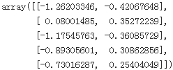
Notice that running PCA multiple times on slightly different datasets may result in different results. In general the only difference is that some axes may be flipped. In this example, PCA using Scikit-Learn gives the same projection as the one given by the SVD approach, except both axes as flipped:
np.allclose( X2D, -X2D_using_svd )![]()
Recover the 3D points projected on the plane (PCA 2D subspace). #reconstruction
Scikit-Learn's PCA class automatically takes care of reversing the mean centering
X3D_inv = pca.inverse_transform(X2D)
np.allclose(X3D_inv, X)![]() # there was some loss of information during the projection step, so the recovered 3D points are not exactly equal to the original 3D points
# there was some loss of information during the projection step, so the recovered 3D points are not exactly equal to the original 3D points
We can compute the reconstruction error:
np.mean( np.sum(np.square(X3D_inv-X), axis=1) )![]()
#reconstruction
The inverse transform in the SVD approach looks like this: #X2D_using_svd = ![]() #W2 = Vt.T[:,:2]
#W2 = Vt.T[:,:2]
# X= X2D_using_svd.dot(W2^T) => X2D_using_svd.dot(Vt[:2,:])
note: the following code does not take care of reversing the mean centering
X3D_inv_using_svd = X2D_using_svd.dot(Vt[:2,:]) # X2D_using_svd = X_centered.dot( Vt.T[:,:2] )The reconstructions from both methods(The inverse transform in the SVD approach and Scikit-Learn's PCA) are not identical because Scikit-Learn's PCA class automatically takes care of reversing the mean centering, but if we subtract the mean ( from the inverse transform in the Scikit-Learn's PCA), we get the same reconstruction:
np.allclose( X3D_inv_using_svd, X3D_inv-pca.mean_ )![]()
pca.mean_ ![]()
round(X[:,0].mean(),8), round(X[:,1].mean(),8), round(X[:,2].mean(),8)![]()
The PCA object gives access to the principal components that it computed:
pca.components_the matrix ![]() , defined as the matrix containing the first d principal components (i.e., the matrix composed of the first d columns of
, defined as the matrix containing the first d principal components (i.e., the matrix composed of the first d columns of ![]()
W2.T![]()
Compare to the first two principal components computed using the SVD method:
# U, s, Vt = np.linalg.svd(X_centered) #Vt contains all the principal components#############
Vt[:2]![]() # Notice how the axes are flipped.
# Notice how the axes are flipped.
Notice how the axes are flipped.
######################### extra materials
Figure 12.1 A synthetic合成的 data sel obtained by taking one of the off-line digit images and creating multiple copies in each of which the digit has undergone 经历 a random displacement置换 and rotation within some larger image field. The resulting images each have 100 * 100 = 10,000 pixels.
We now explore models in which some, or all, of the latent variables are continuous. An important motivation for such models is that many data sets have the property that the data points all lie close to a manifold of much lower dimensionality than that of the original data space. To see why this might arise, consider an artificial data set constructed by taking one of the off-line
digits, represented by a 64 x 64 pixel grey-level image, and embedding it in a larger image of size 100 x 100 by padding with pixels having the value zero (corresponding to white pixels) in which the location and orientation of the digit is varied at random, as illustrated in Figure 12.1. Each of the resulting images is represented by a point in the 100 x 100 = 10,000-dimensional data space. However, across a data set of such images, there are only three degrees of freedom of variability, corresponding to the vertical and horizontal translations and the rotations. The data points will therefore live on a subspace of the data space whose intrinsic dimensionality本质维度 is three. Note that the manifold will be nonlinear because. for instance. if we translate the digit past a particular pixel, that pixel value will go from zero (white) to one (black) and back to zero again. which is clearly a nonlinear function of the digit position. In this example, the translation平移 and rotation parameters are latent variables潜在变量 because we observe only the image vectors and are not told which values of the translation or rotation variables were used to create them.
For real digit image data, there will be a further degree of freedom arising from scaling. Moreover there will be multiple additional degrees of freedom associated with more complex deformations变形 due to the variability in an individual’s writing
as well as the differences in writing styles between individuals. Nevertheless, the number of such degrees of freedom will be small compared to the dimensionality of the data set.
Another example is provided by the oil flow data set, in which (for a given geometrical configuration of the gas, water, and oil phases) there are only two degrees of freedom of variability corresponding to the fraction of oil in the pipe and the fraction of water (the fraction of gas then being determined). Although the data space comprises 12 measurements, a data set of points will lie close to a two-dimensional manifold embedded within this space. In this case, the manifold comprises several distinct segments corresponding to different flow regimes, each such segment being a (noisy) continuous two-dimensional manifold. If our goal is data compression, or density modelling, then there can be benefits in exploiting利用 this manifold structure.
In practice, the data points will not be confined precisely to a smooth low dimensional manifold, and we can interpret the departures偏移 of data points from the manifold as ‘noise’. This leads naturally to a generative view of such models in which we first select a point within the manifold according to some latent variable distribution and then generate an observed data point by adding noise, drawn from some conditional distribution of the data variables given the latent variables.
The simplest continuous latent variable model assumes Gaussian distributions for both the latent and observed variables and makes use of a linear-Gaussian dependence of the observed variables on the state of the latent variables. This leads to a probabilistic formulation概率公式 of the well-known technique of principal component analysis (PCA), as well as to a related model called factor analysis.
In this chapter we will begin with a standard, nonprobabilistic treatment of PCA, and then we show how PCA arises naturally as the maximum likelihood solution最大似然解 to a particular form of linear-Gaussian latent variable model. This probabilistic reformulation brings many advantages, such as the use of EM for parameter estimation, principled extensions to mixtures of PCA models, and Bayesian formulations that allow the number of principal components to be determined automatically from the
data. Finally, we discuss briefly several generalizations of the latent variable concept that go beyond the linear-Gaussian assumption including non-Gaussian latent variables, which leads to the framework of independent component analysis, as well as models having a nonlinear relationship between latent and observed variables.
12.1. Principal Component Analysis
Principal component analysis, or PCA, is a technique that is widely used for applications such as dimensionality reduction, lossy有损耗的 data compression, feature extraction, and data visualization (Jolliffe, 2002). It is also known as the Karhunen-Lo`eve transform.
There are two commonly used definitions of PCA that give rise to the same algorithm. PCA can be defined as the orthogonal projection of the data onto a lower dimensional linear space, known as the principal subspace, such that the variance of the projected data is maximized (Hotelling, 1933). Equivalently, it can be defined as the linear projection that minimizes the average projection cost, defined as the mean squared distance between the data points and their projections (Pearson, 1901). The process of orthogonal projection is illustrated in Figure 12.2. We consider each of these definitions in turn.
########
It seems reasonable to select the axis that preserves the maximum amount of variance(more spread along the selected axis), as it will most likely lose less information than the other projections. Another way to justify this choice is that it is the axis that minimizes the mean squared distance between the original dataset and its projection onto that axis. This is the rather simple idea behind PCA.
########
Figure 12.2 Principal component analysis seeks a space of lower dimensionality, known as the principal subspace and denoted by the magenta紫红色的 line, such that the orthogonal projection of the data points (red dots) onto this subspace maximizes the variance of the projected points (green dots). An alternative definition of PCA is based on minimizing the sum-of-squares of the projection errors, indicated by the blue lines.
12.1.1 Maximum variance formulation
Consider a data set of observations ![]() where n = 1, . . . , N, and
where n = 1, . . . , N, and ![]() is a Euclidean variable with dimensionality D. Our goal is to project the data onto a space having dimensionality M
is a Euclidean variable with dimensionality D. Our goal is to project the data onto a space having dimensionality M
To begin with, consider the projection onto a one-dimensional space (M = 1). We can define the direction of this space using a D-dimensional vector ![]() , which for convenience (and without loss of generality) we shall choose to be a unit vector so that
, which for convenience (and without loss of generality) we shall choose to be a unit vector so that ![]() = 1 (note that we are only interested in the direction defined by
= 1 (note that we are only interested in the direction defined by ![]() , not in the magnitude of
, not in the magnitude of ![]() itself). Each data point
itself). Each data point ![]() is then projected onto a scalar value
is then projected onto a scalar value ![]() . The mean of the projected data is
. The mean of the projected data is ![]() where
where ![]() is the sample set mean given by
is the sample set mean given by  (12.1)
and the variance of the projected data is given by  (12.2)
where S is the data covariance 协方差 matrix defined by  (12.3)
We now maximize the projected variance ![]() with respect to
with respect to ![]() . Clearly, this has to be a constrained maximization to prevent
. Clearly, this has to be a constrained maximization to prevent ![]() . The appropriate constraint comes from the normalization condition归一化条件
. The appropriate constraint comes from the normalization condition归一化条件 ![]() = 1. To enforce this constraint, we introduce a Lagrange multiplier that we shall denote by
= 1. To enforce this constraint, we introduce a Lagrange multiplier that we shall denote by ![]() , and then make an unconstrained maximization of
, and then make an unconstrained maximization of ![]() (12.4)
(12.4)
By setting the derivative with respect to ![]() equal to zero, we see that this quantity will have a stationary point驻点 when
equal to zero, we see that this quantity will have a stationary point驻点 when ![]() (12.5) which says that
(12.5) which says that ![]() must be an eigenvector 特征向量 of S. If we left-multiply by
must be an eigenvector 特征向量 of S. If we left-multiply by ![]() and make use of
and make use of ![]() = 1, we see that the variance is given by
= 1, we see that the variance is given by ![]() (12.6)
(12.6)
and so the variance will be a maximum when we set ![]() equal to the eigenvector having the largest eigenvalue
equal to the eigenvector having the largest eigenvalue ![]() . This eigenvector is known as the first principal component.
. This eigenvector is known as the first principal component.
We can define additional principal components in an incremental fashion方式 by choosing each new direction to be that which maximizes the projected variance amongst all possible directions orthogonal to those already considered. If we consider the general case of an M-dimensional projection space, the optimal linear projection for which the variance of the projected data is maximized is now defined by the M eigenvectors ![]() of the data covariance matrix S corresponding to the M largest eigenvalues
of the data covariance matrix S corresponding to the M largest eigenvalues ![]() . This is easily shown using proof by induction.
. This is easily shown using proof by induction.
To summarize, principal component analysis involves evaluating the mean ![]() and the covariance matrix S of the data set and then finding the M eigenvectors of S corresponding to the M largest eigenvalues. Algorithms for finding eigenvectors and eigenvalues, as well as additional theorems related to eigenvector decomposition, can be found in Golub and Van Loan (1996). Note that the computational cost of computing the full eigenvector decomposition for a matrix of size D x D is
and the covariance matrix S of the data set and then finding the M eigenvectors of S corresponding to the M largest eigenvalues. Algorithms for finding eigenvectors and eigenvalues, as well as additional theorems related to eigenvector decomposition, can be found in Golub and Van Loan (1996). Note that the computational cost of computing the full eigenvector decomposition for a matrix of size D x D is ![]() .If we plan to project our data onto the first M principal components, then we only need to find the first M eigenvalues and eigenvectors. This can be done with more efficient techniques, such as the power method (Golub and Van Loan, 1996), that scale like
.If we plan to project our data onto the first M principal components, then we only need to find the first M eigenvalues and eigenvectors. This can be done with more efficient techniques, such as the power method (Golub and Van Loan, 1996), that scale like ![]() , or alternatively we can make use of the EM algorithm.
, or alternatively we can make use of the EM algorithm.
12.1.2 Minimum-error formulation
We now discuss an alternative formulation of PCA based on projection error minimization. To do this, we introduce a complete orthonormal set of D-dimensional basis vectors {![]() } where i = 1, ... , D that satisfy
} where i = 1, ... , D that satisfy ![]() (12.7)
(12.7)
Because this basis is complete, each data point can be represented exactly by a linear combination of the basis vectors  (12.8)
where the coefficients ![]()
![]() will be different for different data points. This simply corresponds to a rotation of the coordinate system to a new system defined by the {
will be different for different data points. This simply corresponds to a rotation of the coordinate system to a new system defined by the {![]() }, and the original D components {
}, and the original D components {![]() } are replaced by an equivalent
} are replaced by an equivalent
set {![]() }. Taking the inner product with
}. Taking the inner product with ![]() , and making use of the orthonormality property, we obtain
, and making use of the orthonormality property, we obtain ![]() , and so without loss of generality we can write
, and so without loss of generality we can write  (12.9)
#########################https://docs.scipy.org/doc/numpy/reference/generated/numpy.linalg.svd.html
numpy.linalg.svd
numpy.linalg.svd(a, full_matrices=True, compute_uv=True, hermitian=False)
Singular Value Decomposition.奇异值分解
When a is a 2D array, it is factorized as u @ np.diag(s) @ vh = (u * s) @ vh, where u and vh are 2D unitary单位的 arrays and s is a 1D array of a’s singular values. When a is higher-dimensional, SVD is applied in stacked mode as explained below.
#########################
https://blog.csdn.net/Linli522362242/article/details/105196037
Explained Variance Ratio
Another very useful piece of information is the explained variance ratio of each principal component, available via the explained_variance_ratio_ variable. It indicates the proportion of the dataset’s variance that lies along the axis of each principal component. For example, let’s look at the explained variance ratios of the first two components of the 3D dataset represented in Figure 8-2:
Now let's look at the explained variance ratio:
# from sklearn.decomposition import PCA

# pca = PCA( n_components=2 )
# X2D = pca.fit_transform(X)

pca.explained_variance_ratio_ #Percentage of variance explained by each of the selected components.![]() #??????????? see below
#??????????? see below
This tells you that 84.2% of the dataset’s variance lies along the first axis, and 14.6% lies along the second axis. This leaves less than 1.2% for the third axis, so it is reasonable to assume that it probably carries little information.
By projecting down to 2D, we lost about 1.1% of the variance:
1-pca.explained_variance_ratio_.sum()![]()
Here is how to compute the explained variance ratio using the SVD approach (recall that s is the diagonal of the matrix S):
s contains all singular values # U, s, Vt = np.linalg.svd(X_centered)
np.square(s) == eigenvalues![]() ; OR one singular value
; OR one singular value ![]()
The variance explained ratio(方差解释比率或者方差贡献率) of an eigenvalue![]() is simply the fraction of an eigenvalue
is simply the fraction of an eigenvalue![]() and the total sum of the eigenvalues:
and the total sum of the eigenvalues:
np.square(s) / np.square(s).sum()![]()
s![]()
np.diag(s)
####################################
# The amount of variance explained by each of the selected components.
pca.explained_variance_ # Equal to n_components largest eigenvalues of the covariance matrix of X.
pca.explained_variance_ #The amount of variance explained by each of the selected components.![]()
0.77830975/(0.77830975 + 0.1351726)![]() xxxxxxxxxxxxxxx
xxxxxxxxxxxxxxx
0.1351726/(0.77830975 + 0.1351726)![]() xxxxxxxxxxxxxxxxxx
xxxxxxxxxxxxxxxxxx
from sklearn.decomposition import PCA

pca = PCA() # n_components: if n_components is not set all components are kept
X2D = pca.fit_transform(X)

pca.explained_variance_ratio_![]()
![]()
![]()
![]()
pca.explained_variance_![]()
0.77830975/(0.77830975+ 0.1351726 + 0.01034272)![]()
![]()
![]()
![]()
0.1351726/(0.77830975+ 0.1351726 + 0.01034272)![]()
![]()
![]()
![]()
####################################
Choosing the Right Number of Dimensions
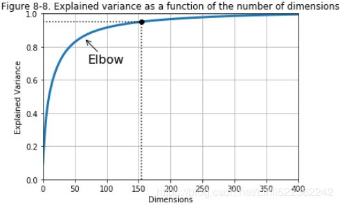
Instead of arbitrarily choosing the number of dimensions to reduce down to, it is generally preferable to choose the number of dimensions that add up to a sufficiently large portion of the variance (e.g., 95%). Unless, of course, you are reducing dimensionality for data visualization—in that case you will generally want to reduce the dimensionality down to 2 or 3.
The following code computes PCA without reducing dimensionality, then computes the minimum number of dimensions required to preserve 95% of the training set’s variance:
from sklearn.datasets import fetch_openml
from sklearn.model_selection import train_test_split

mnist = fetch_openml('mnist_784', version=1)
mnist.target = mnist.target.astype(np.uint8)

X = mnist['data']
y = mnist['target']

# X_train.shape=>(52500, 784) #X_test.shape=>(17500, 784)
X_train, X_test, y_train, y_test = train_test_split(X,y) # default test_size=0.25
pca = PCA() #computes PCA without reducing dimensionality
pca.fit(X_train)
cumsum = np.cumsum(pca.explained_variance_ratio_)
d = np.argmax(cumsum>=0.95)+1 #computes the minimum number of dimensions required to preserve 95% of the training set’s variance
d![]()
You could then set n_components=d and run PCA again. However, there is a much better option: instead of specifying the number of principal components you want to preserve, you can set n_components to be a float between 0.0 and 1.0, indicating the ratio of variance you wish to preserve:
pca = PCA(n_components=0.95)
X_reduced = pca.fit_transform(X_train)
X_reduced.shape![]()
Yet another option is to plot the explained variance as a function of the number of dimensions (simply plot cumsum; see Figure 8-8). There will usually be an elbow(肘部) in the curve, where the explained variance stops growing fast. You can think of this as the intrinsic dimensionality of the dataset. In this case, you can see that reducing the dimensionality down to about 100 dimensions wouldn’t lose too much explained variance.
plt.figure( figsize=(6,4) )
plt.plot( cumsum, linewidth=3 )
plt.axis([0,400, 0,1])
plt.xlabel("Dimensions")
plt.ylabel("Explained Variance")
plt.plot( [d,d], [0,0.95], "k:" ) #d: the minimum number of dimensions required to preserve 95% of the training set’s variance
plt.plot( [0,d], [0.95,0.95], "k:" ) #95% of the training set’s variance
plt.plot( d,0.95, "ko" )
plt.annotate( "Elbow", xy=(65,0.85), xytext=(70,0.7), arrowprops=dict(arrowstyle="->"), fontsize=16 )
plt.grid(True)

plt.show()
PCA for Compression
Obviously after dimensionality reduction, the training set takes up much less space. For example, try applying PCA to the MNIST dataset while preserving 95% of its variance. You should find that each instance will have just over 150 features, instead of the original 784 features. So while most of the variance is preserved, the dataset is now less than还不到 20% of its original size(154/784)! This is a reasonable compression ratio, and you can see how this can speed up a classification algorithm (such as an SVM classifier) tremendously极大地.
It is also possible to decompress the reduced dataset back to 784 dimensions by applying the inverse transformation of the PCA projection. Of course this won’t give you back the original data, since the projection lost a bit of information (within the 5% variance that was dropped), but it will likely be quite close to the original data. The mean squared distance between the original data and the reconstructed data (compressed and then decompressed) is called the reconstruction error. For example, the following code compresses the MNIST dataset down to 154 dimensions, then uses the inverse_transform() method to decompress it back to 784 dimensions. Figure 8-9 shows a few digits from the original training set (on the left), and the corresponding digits after compression and decompression. You can see that there is a slight image quality loss, but the digits are still mostly intact完好无损的.
pca = PCA(n_components=0.95)
X_reduced = pca.fit_transform(X_train)
# pca.n_components_ #154
# np.sum( pca.explained_variance_ratio_ ) # 0.9503207480330471

pca = PCA( n_components=154 )
X_reduced = pca.fit_transform( X_train )
X_recovered = pca.inverse_transform( X_reduced )


import matplotlib as mpl

def plot_digits( instances, images_per_row=5, **options ):
    size=28
    images_per_row = min( len(instances), images_per_row )
    n_rows = ( len(instances)-1 ) //images_per_row + 1 #or (49-1)//49+1=5 instead 49//10=4 : need +1
                                                       #or (52-1)//10+1=6 instead 52//10=5 # need +1
                                                    #or (50-1)//10+1=5 instead (50)//10+1=6 need 50-1
    images = [ instance.reshape(size,size) for instance in instances ] # each instance: 28x28 ##ndarray
    row_images = []
    #process empty on the last row or the number of last row images != images_per_row
    if n_rows * images_per_row >len(instances) : #fill with 28*28 0's
        n_empty = n_rows * images_per_row - len(instances)
                                  #hint:tile horizontal                           #Dimension
        images.append( np.zeros( (size,size*n_empty) ) )#wrong:np.zeros((size,size))*n_empty==np.zeros((size,size))
                                            #wrong:np.zeros((size,size)*n_empty) #2^n_empty dimensions
        #images.append( np.tile( np.zeros((size,size)),n_empty ) )
    for row in range( n_rows ):                  #index[0]  : image[0]...image[9] in row 0
        rimages = images[ row*images_per_row: (row+1)*images_per_row ] #block or subgroup
        row_images.append( np.concatenate(rimages, axis=1) ) #images per row
    image = np.concatenate( row_images, axis=0 )
    plt.imshow( image, cmap = mpl.cm.binary, **options )
    plt.axis("off")


plt.figure( figsize=(7,4) )

plt.subplot(121)
plot_digits(X_train[::2100])  # 52500/2100=25=5*5
plt.title("Original", fontsize=16)

plt.subplot(122)
plot_digits(X_recovered[::2100])
plt.title("Compressed", fontsize=16)
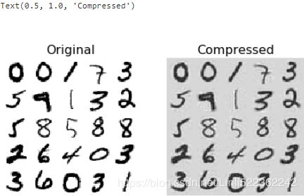
Figure 8-9. MNIST compression preserving 95% of the variance
X_reduced_pca = X_reducedThe equation of the inverse transformation is shown in Equation 8-3.
Equation 8-3. PCA inverse transformation, back to the original number of dimensions![]()
Equation 8-2. Projecting the training set down to d dimensions![]() #W2 = Vt.T[:, :2]
#W2 = Vt.T[:, :2]
Incremental PCA
One problem with the preceding implementation of PCA is that it requires the whole training set to fit in memory in order for the SVD algorithm to run. Fortunately, Incremental PCA (IPCA) algorithms have been developed: you can split the training set into mini-batches and feed an IPCA algorithm one minibatch at a time. This is useful for large training sets, and also to apply PCA online (i.e., on the fly, as new
instances arrive即在新实例到达时即时运行).
The following code splits the MNIST dataset into 100 mini-batches (using NumPy’s array_split() function) and feeds them to Scikit-Learn’s IncrementalPCA class to reduce the dimensionality of the MNIST dataset down to 154 dimensions (just like before). Note that you must call the partial_fit() method with each mini-batch rather than the fit() method with the whole training set:
partial_fit(self, X, y=None, check_input=True) : Incremental fit with X. All of X is processed as a single batch
fit(self, X, y=None) : Fit the model with X, using minibatches of size batch_size.
from sklearn.decomposition import IncrementalPCA

n_batches = 100
inc_pca = IncrementalPCA( n_components=154 )
for X_batch in np.array_split( X_train, n_batches ):
    #print( ".", end="") # not shown in the book
    inc_pca.partial_fit( X_batch )

X_reduced = inc_pca.transform(X_train)

X_recovered_inc_pca = inc_pca.inverse_transform( X_reduced )
X_reduced_inc_pca = X_reduced

plt.figure( figsize=(7,4) )

plt.subplot( 121 )
plot_digits( X_train[::2100] )
plt.title("Original", fontsize=16)

plt.subplot( 122 )
plot_digits( X_recovered_inc_pca[::2100] )
plt.title("Compressed_Inc_PCA", fontsize=16)

plt.tight_layout()
Let's compare the results of transforming MNIST using regular PCA and incremental PCA. First, the means are equal:
np.allclose(pca.mean_, inc_pca.mean_)![]()
X_train.mean(axis=0)pca.mean_But the results(reduced dimension-dataset) are not exactly identical. Incremental PCA gives a very good approximate solution(regular PCA is that it requires the whole training set to fit in memory in order for the SVD algorithm to run), but it's not perfect:
np.allclose( X_reduced_pca, X_reduced_inc_pca )![]()
Alternatively, you can use NumPy’s memmap class, which allows you to manipulate a large array stored in a binary file on disk as if it were entirely in memory; the class loads only the data it needs in memory, when it needs it. Since the IncrementalPCA class uses only a small part of the array at any given time, the memory usage remains under control. This makes it possible to call the usual fit() method, as you can see in the following code:
Using memmap()
Let's create the memmap() structure and copy the MNIST data into it. This would typically be done by a first program:
filename = "my_mnist.data"
m,n = X_train.shape

X_mm = np.memmap( filename, dtype="float32", mode="write", shape=(m,n) )
X_mm[:] = X_train #copy the MNIST data into it
Now deleting the memmap() object will trigger its Python finalizer, which ensures that the data is saved to disk.
del X_mm
Next, another program would load the data and use it for training:
X_mm = np.memmap( filename, dtype="float32", mode="readonly", shape=(m,n) )

batch_size = m//n_batches  #n_batches=100 #==>batch_size=525
inc_pca = IncrementalPCA( n_components=154, batch_size=batch_size )
inc_pca.fit(X_mm)![]()
Randomized PCA
Scikit-Learn offers yet another option to perform PCA, called Randomized PCA. This is a stochastic algorithm that quickly finds an approximation近似值 of the first d principal components. Its computational complexity is O(m × d^2) + O(d^3), instead of O(m × n^2) + O(n^3), so it is dramatically显著地 faster than the previous algorithms when d is much smaller than n.
rnd_pca = PCA(n_components=154, svd_solver="randomized", random_state=42)
X_reduced = rnd_pca.fit_transform(X_train)
Time complexity
Let's time regular PCA against Incremental PCA and Randomized PCA, for various number of principal components:
import time

for n_components in (2,10,154):
    print("n_components=", n_components)
    regular_pca = PCA( n_components=n_components )
    inc_pca = IncrementalPCA( n_components=n_components, batch_size=500 )
    rnd_pca = PCA( n_components=n_components, random_state=42, svd_solver="randomized" )

    for pca in (regular_pca, inc_pca, rnd_pca):
        t1 = time.time()
        pca.fit(X_train)
        t2 = time.time()
        print( "     {}: {:.1f} seconds".format(pca.__class__.__name__, t2-t1) )
Now let's compare PCA and Randomized PCA for datasets of different sizes (number of instances):
times_rpca = []
times_pca = []

sizes = [1000, 10000, 20000, 30000, 40000, 50000, 70000, 100000, 200000, 500000]
for n_samples in sizes:
    X = np.random.randn( n_samples, 5 )
    pca = PCA( n_components=2, svd_solver="randomized", random_state=42 )
    t1 = time.time()
    pca.fit(X)
    t2 = time.time()
    times_rpca.append( t2-t1 )

    pca = PCA(n_components=2) #regular PCA
    t1 = time.time()
    pca.fit(X)
    t2 = time.time()
    times_pca.append( t2-t1 )

plt.plot( sizes, times_rpca, "b-o", label="Randomized PCA")
plt.plot( sizes, times_pca, "r-s", label="PCA")
plt.xlabel("n_samples")
plt.ylabel("Training time")
plt.legend(loc="upper left")
plt.title("PCA and Randomized PCA time complexity")
plt.show()
times_rpca = []
times_pca = []
sizes = [1000, 2000, 3000, 4000, 5000, 6000]
for n_features in sizes:
X = np.random.randn(2000, n_features)
pca = PCA(n_components=2, random_state=42, svd_solver="randomized")
t1 = time.time()
pca.fit(X)
t2 = time.time()
times_rpca.append(t2-t1)
pca = PCA(n_components=2)
t1 = time.time()
pca.fit(X)
t2 = time.time()
times_pca.append(t2-t1)
plt.plot(sizes, times_rpca, "b-o", label="RandomizedPCA")
plt.plot(sizes, times_pca, "r-s", label="PCA")
plt.xlabel("n_features")
plt.ylabel("Training time")
plt.legend(loc="upper left")
plt.title("PCA and Randomized PCA time complexity")
Kernel PCA
In Cp5 https://blog.csdn.net/Linli522362242/article/details/104403372 we discussed the kernel trick, a mathematical technique that implicitly maps instances into a very high-dimensional space (called the feature space), enabling nonlinear classification and regression with Support Vector Machines. Recall that a linear decision boundary in the high-dimensional feature space corresponds to a complex nonlinear decision boundary in the original space. It turns out that the same trick can be applied to PCA, making it possible to perform complex nonlinear projections for dimensionality reduction. This is called Kernel PCA (kPCA). It is often good at preserving clusters of instances after projection, or sometimes even unrolling datasets that lie close to a twisted manifold.
For example, the following code uses Scikit-Learn’s KernelPCA class to perform kPCA with an RBF kernel (see Cp5 for more details about the RBF kernel and the other kernels):
X,t = make_swiss_roll( n_samples=1000, noise=0.2, random_state=42 )

from sklearn.decomposition import KernelPCA

rbf_pca = KernelPCA( n_components=2, kernel="rbf", gamma=0.04)
X_reduced = rbf_pca.fit_transform(X)
#############################################################https://blog.csdn.net/Linli522362242/article/details/104280075
Kernelized SVM
Suppose you want to apply a 2nd-degree polynomial transformation to a two dimensional training set (such as the moons training set), then train a linear SVM classifier on the transformed training set. Equation 5-8 shows the 2nd-degree polynomial mapping function ϕ that you want to apply.
Equation 5-8. Second-degree polynomial mapping 
two-dimensional input space x = ![]()
Notice that the transformed vector is three-dimensional instead of two-dimensional. Now let's look at what happens to a couple of two-dimensional vectors, a and b, if we apply this 2nd-degree polynomial mapping and then compute the dot product of the transformed vectors (See Equation 5-9).
Equation 5-9. Kernel trick for a 2nd-degree polynomial mapping ![]()
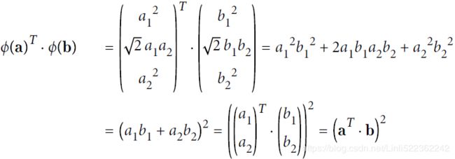
How about that? The dot product of the transformed vectors![]() is equal to the square of the dot product of the original vectors:
is equal to the square of the dot product of the original vectors: ![]() .
.
The function ![]() is called a 2nd-degree polynomial kernel. In Machine Learning, a kernel is a function capable of computing the dot product
is called a 2nd-degree polynomial kernel. In Machine Learning, a kernel is a function capable of computing the dot product ![]() based only on the original vectors a and b, without having to compute (or even to know about) the transformation ϕ. Equation 5-10 lists some of the most commonly used kernels.
based only on the original vectors a and b, without having to compute (or even to know about) the transformation ϕ. Equation 5-10 lists some of the most commonly used kernels.![]()
3 The Behavior of the Sigmoid Kernel
tanh是双曲函数中的一个,tanh()为双曲正切。在数学中,双曲正切“tanh”是由双曲正弦和双曲余弦这两种基本双曲函数推导而来。
公式 
定义域和值域
函数:y=tanh x;定义域:R,值域:(-1,1)。y=tanh x是一个奇函数,其函数图像为过原点并且穿越Ⅰ、Ⅲ象限的严格单调递增曲线,其图像被限制在两水平渐近线y=1和y=-1之间。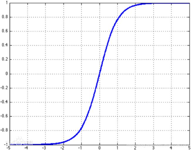
In this section, we consider the sigmoid kernel ![]() , which takes two parameters: a and r. For a > 0, we can view a as a scaling parameter缩放参数 of the input data, and r as a shifting parameter移位参数 that controls the threshold of mapping. For a < 0, the dot-product of the input data is not only scaled but reversed. In the following table we summarize the behavior in different parameter combinations, which will be discussed in the rest of this section. It concludes that the first case, a > 0 and r < 0, is more suitable for the sigmoid kernel
, which takes two parameters: a and r. For a > 0, we can view a as a scaling parameter缩放参数 of the input data, and r as a shifting parameter移位参数 that controls the threshold of mapping. For a < 0, the dot-product of the input data is not only scaled but reversed. In the following table we summarize the behavior in different parameter combinations, which will be discussed in the rest of this section. It concludes that the first case, a > 0 and r < 0, is more suitable for the sigmoid kernel
#############################################################
from sklearn.decomposition import KernelPCA

lin_pca = KernelPCA( n_components=2, kernel="linear", fit_inverse_transform=True )
rbf_pca = KernelPCA( n_components=2, kernel="rbf", gamma=0.0433, fit_inverse_transform=True)
                                                                   # coef0== r as a shifting parameter that controls the threshold of mapping
sig_pca = KernelPCA( n_components=2, kernel="sigmoid", gamma=0.001, coef0=1, fit_inverse_transform=True)

y = t>6.9

plt.figure( figsize=(14,4) )
for subplot, pca, title in ( (131, lin_pca, "Linear kernel"),
                            (132, rbf_pca, "RBF kernel, $\gamma=0.04$"),
                            (133, sig_pca, "Sigmoid kernel, $\gamma=10^{-3}, r=1$")
                           ):
    X_reduced = pca.fit_transform(X)
    if subplot==132:
        X_reduced_rbf = X_reduced ########################

    plt.subplot( subplot )
    plt.title(title, fontsize=14)
    plt.scatter(X_reduced[:,0], X_reduced[:,1], c=t, cmap=plt.cm.hot)
    plt.xlabel("$z_1$", fontsize=18)
    if subplot==131:
        plt.ylabel("$z_2$", fontsize=18, rotation=0)
    plt.grid(True)
plt.show()
Figure 8-10 shows the Swiss roll, reduced to two dimensions using a linear kernel (equivalent to simply using the PCA class), an RBF kernel, and a sigmoid kernel (Logistic). # in Reduced space
plt.figure( figsize=(6,5) )

# uses GridSearchCV to find the best kernel="rbf" and gamma value=0.043333333333333335 for kPCA
# fit_inverse_transform=True:
#           projected instances as the training set and the original instances as the targets
# rbf_pca = KernelPCA( n_components=2, kernel="rbf", gamma=0.0433, fit_inverse_transform=True)
# X_reduced_rbf = rbf_pca.fit_transform(X) # train a supervised regression model
X_inverse = rbf_pca.inverse_transform(X_reduced_rbf) #X_preimage

ax = plt.subplot(111, projection='3d')
ax.view_init( 10,-70 )
ax.scatter( X_inverse[:,0], X_inverse[:,1], X_inverse[:,2], c=t, cmap=plt.cm.hot, marker="x")
ax.set_xlabel("")
ax.set_ylabel("")
ax.set_zlabel("")
ax.set_xticklabels([])
ax.set_yticklabels([])
ax.set_zticklabels([])
plt.title("Reconstruction Pre-image")
plt.show()
# uses GridSearchCV to find the best kernel="rbf" and gamma value=0.043333333333333335 for kPCA
# fit_inverse_transform=True:
# projected instances as the training set and the original instances as the targets
# rbf_pca = KernelPCA( n_components=2, kernel="rbf", gamma=0.0433, fit_inverse_transform=True)
X_reduced = rbf_pca.fit_transform(X)
plt.figure( figsize=(16,5) )
plt.subplot(132)
plt.scatter(X_reduced[:,0], X_reduced[:,1]*-1, c=t, cmap=plt.cm.hot, marker="x")
plt.xlabel("$z_1$", fontsize=18)
plt.ylabel("$z_2$", fontsize=18)
plt.grid(True)Reduced space
 <== X_reduced[:,1]*-1<==
###############################
NOTE
The direction of the principal components(eigenvectors) is not stable: if you perturb打乱 the training set slightly and run PCA again, some of the new PCs(Principal Components) may point in the opposite direction of the original PCs. However, they will generally still lie on the same axes. In some cases, a pair of PCs may even rotate or swap, but the plane they define will generally remain the same.
###############################
Selecting a Kernel and Tuning Hyperparameters
As kPCA is an unsupervised learning algorithm, there is no obvious performance measure to help you select the best kernel and hyperparameter values. However, dimensionality reduction is often a preparation step for a supervised learning task (e.g., classification), so you can simply use grid search to select the kernel and hyperparameters that lead to the best performance on that task.
For example, the following code creates a two-step pipeline, first reducing dimensionality to two dimensions using kPCA, then applying Logistic Regression for classification. Then it uses GridSearchCV to find the best kernel and gamma value for kPCA in order to get the best classification accuracy at the end of the pipeline:
from sklearn.model_selection import GridSearchCV
from sklearn.linear_model import LogisticRegression
from sklearn.pipeline import Pipeline

clf = Pipeline([
    ("kpca", KernelPCA( n_components=2 )),
    ("log_reg", LogisticRegression(solver="lbfgs"))
])

param_grid = [{
    "kpca__gamma": np.linspace(0.03, 0.05, 10), #Note: two continue underline
    "kpca__kernel": ["rbf", "sigmoid"]
}]

grid_search = GridSearchCV(clf, param_grid, cv=3)
grid_search.fit(X,y)
####################################
from sklearn.model_selection import GridSearchCV
from sklearn.linear_model import LogisticRegression
from sklearn.pipeline import Pipeline

clf = Pipeline([
    ("kpca", KernelPCA( n_components=2 )),
    ("log_reg", LogisticRegression(solver="lbfgs"))
])

param_grid = [{
    "kpca_gamma": np.linspace(0.03, 0.05, 10), #Note: two continue underline
    "kpca_kernel": ["rbf", "sigmoid"]
}]

grid_search = GridSearchCV(clf, param_grid, cv=3)
grid_search.fit(X,y)
---------------------------------------------------------------------------
ValueError Traceback (most recent call last)
in
14
15 grid_search = GridSearchCV(clf, param_grid, cv=3)
---> 16 grid_search.fit(X,y)
... ...
ValueError: Invalid parameter kpca_gamma for estimator Pipeline(memory=None,
steps=[('kpca',
KernelPCA(alpha=1.0, coef0=1, copy_X=True, degree=3,
eigen_solver='auto', fit_inverse_transform=False,
gamma=None, kernel='linear', kernel_params=None,
max_iter=None, n_components=2, n_jobs=None,
random_state=None, remove_zero_eig=False, tol=0)),
('log_reg',
LogisticRegression(C=1.0, class_weight=None, dual=False,
fit_intercept=True, intercept_scaling=1,
l1_ratio=None, max_iter=100,
multi_class='auto', n_jobs=None,
penalty='l2', random_state=None,
solver='lbfgs', tol=0.0001, verbose=0,
warm_start=False))],
verbose=False). Check the list of available parameters with `estimator.get_params().keys()`.
####################################
The best kernel and hyperparameters are then available through the best_params_variable:
print(grid_search.best_params_) ![]()
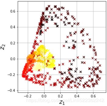
Another approach, this time entirely unsupervised, is to select the kernel and hyperparameters that yield the lowest reconstruction error. However, reconstruction is not as easy as with linear PCA. Here’s why. Figure 8-11 shows the original Swiss roll 3D dataset (top left), and the resulting 2D dataset after kPCA is applied using an RBF kernel (top right). Thanks to the kernel trick, this is mathematically equivalent to mapping the training set to an infinite-dimensional feature space (bottom right) using the feature map φ, then projecting the transformed training set down to 2D using linear PCA. Notice that if we could invert the linear PCA step for a given instance in the reduced space, the reconstructed point would lie in feature space, not in the original space (e.g., like the one represented by an x in the diagram). Since the feature space is infinite-dimensional, we cannot compute the reconstructed point, and therefore we cannot compute the true reconstruction error. Fortunately, it is possible to find a point in the original space that would map close to the reconstructed point. This is called the reconstruction pre-image重建前图像. Once you have this pre-image, you can measure its(pre-image's) squared distance to the original instance. You can then select the kernel and hyperparameters that minimize this reconstruction pre-image error.
Figure 8-11. Kernel PCA and the reconstruction pre-image error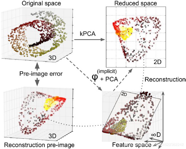
You may be wondering how to perform this reconstruction. One solution is to train a supervised regression model, with the projected instances as the training set and the original instances as the targets. Scikit-Learn will do this automatically if you set fit_inverse_transform=True, as shown in the following code:
# fit_inverse_transform=True:
#           projected instances as the training set and the original instances as the targets
rbf_pca = KernelPCA( n_components=2, kernel="rbf", gamma=0.0433, fit_inverse_transform=True )
X_reduced = rbf_pca.fit_transform(X) #train a supervised regression model
X_preimage = rbf_pca.inverse_transform(X_reduced)


#You can then compute the reconstruction pre-image error:
from sklearn.metrics import mean_squared_error

mean_squared_error(X, X_preimage)![]()
Now you can use grid search with cross-validation to find the kernel and hyperparameters that minimize this pre-image reconstruction error.???
LLE
Locally Linear Embedding (LLE)局部线性嵌入 is another very powerful nonlinear dimensionality reduction (NLDR) technique. It is a Manifold Learning technique that does not rely on projections like the previous algorithms. In a nutshell简而言之, LLE works by first measuring how each training instance linearly relates to its closest neighbors (c.n.), and then
looking for a low-dimensional representation of the training set where these local relationships are best preserved (more details shortly). This makes it particularly good at unrolling twisted manifolds, especially when there is not too much noise.
For example, the following code uses Scikit-Learn’s LocallyLinearEmbedding class to unroll the Swiss roll. The resulting 2D dataset is shown in Figure 8-12. As you can see, the Swiss roll is completely unrolled and the distances between instances are locally well preserved. However, distances are not preserved on a larger scale距离不能在较大范围内保留的很好: the left part of the unrolled Swiss roll is squeezed被挤压, while the right part is stretched被拉长. Nevertheless,
LLE did a pretty good job at modeling the manifold.
# t is the postion after unrolling the swiss roll
X,t = make_swiss_roll( n_samples = 1000, noise=0.2, random_state=41 )


from sklearn.manifold import LocallyLinearEmbedding

lle = LocallyLinearEmbedding(n_components=2, n_neighbors=10, random_state=42)
X_reduced = lle.fit_transform(X)

plt.title("Unrolled swiss roll using LLE", fontsize=14)
plt.scatter(X_reduced[:,0], X_reduced[:,1], c=t, cmap=plt.cm.hot)
plt.xlabel("$z_1$", fontsize=18)
plt.ylabel("$z_2$", fontsize=18)
plt.axis([-0.065, 0.055, -0.1, 0.12])
plt.grid(True)

plt.show()
#####################################################################
https://www.cnblogs.com/pinard/p/6266408.html
局部线性嵌入(Locally Linear Embedding,以下简称LLE)也是非常重要的降维方法。和传统的PCA,LDA等关注样本方差的降维方法相比,LLE关注于降维时保持样本局部的线性特征,由于LLE在降维时保持了样本的局部特征,它广泛的用于图像图像识别,高维数据可视化等领域。下面我们就对LLE的原理做一个总结。
1. 流形学习概述
LLE属于流形学习(Manifold Learning)的一种。因此我们首先看看什么是流形学习。流形学习是一大类基于流形的框架。数学意义上的流形比较抽象,不过我们可以认为LLE中的流形是一个不闭合的曲面。这个流形曲面有数据分布比较均匀,且比较稠密的特征,有点像流水的味道。基于流行的降维算法就是将流形从高维到低维的降维过程,在降维的过程中我们希望流形在高维的一些特征可以得到保留。
一个形象的流形降维过程如下图。我们有一块卷起来的布,我们希望将其展开到一个二维平面,我们希望展开后的布能够在局部保持布结构的特征,其实也就是将其展开的过程,就想两个人将其拉开一样。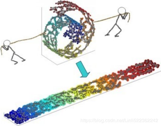
在局部保持布结构的特征,或者说数据特征的方法有很多种,不同的保持方法对应不同的流形算法。比如等距映射(ISOMAP)算法在降维后希望保持样本之间的测地距离而不是欧式距离,因为测地距离更能反映样本之间在流形中的真实距离。
但是等距映射算法有一个问题就是他要找所有样本全局的最优解,当数据量很大,样本维度很高时,计算非常的耗时,鉴于这个问题,LLE通过放弃所有样本全局最优的降维,只是通过保证局部最优来降维。同时假设样本集在局部是满足线性关系的,进一步减少的降维的计算量。
2. LLE思想
现在我们来看看LLE的算法思想。
LLE首先假设数据在较小的局部是线性的,也就是说,某一个数据可以由它邻域中的几个样本来线性表示。比如我们有一个样本![]() ,我们在它的原始高维邻域里用K-近邻思想找到和它最近的三个样本
,我们在它的原始高维邻域里用K-近邻思想找到和它最近的三个样本![]() . 然后我们假设
. 然后我们假设![]() 可以由
可以由![]() 线性表示,即:
线性表示,即:
![]()
其中,![]() 为权重系数。在我们通过LLE降维后,我们希望
为权重系数。在我们通过LLE降维后,我们希望![]() 在低维空间对应的投影
在低维空间对应的投影![]() 和
和![]() 对应的投影
对应的投影![]() 也尽量保持同样的线性关系,即
也尽量保持同样的线性关系,即
![]()
也就是说,投影前后线性关系的权重系数![]() 是尽量不变或者最小改变的。
是尽量不变或者最小改变的。
从上面可以看出,线性关系只在样本的附近起作用,离样本远的样本对局部的线性关系没有影响,因此降维的复杂度降低了很多。
下面我们推导LLE算法的过程。
3. LLE算法推导
对于LLE算法,我们首先要确定邻域大小的选择,即我们需要多少个邻域样本来线性表示某个样本。假设这个值为k。我们可以通过和KNN一样的思想通过距离度量比如欧式距离来选择某样本的k个最近邻。
step 2: 求解权重系数矩阵
在寻找到某个样本的![]() 的k个最近邻之后我们就需要找到找到
的k个最近邻之后我们就需要找到找到![]() 和这k个最近邻之间的线性关系,也就是要找到线性关系的权重系数。找线性关系,这显然是一个回归问题。假设我们有m个n维样本
和这k个最近邻之间的线性关系,也就是要找到线性关系的权重系数。找线性关系,这显然是一个回归问题。假设我们有m个n维样本![]() ,我们可以用均方差作为回归问题的损失函数:即:
,我们可以用均方差作为回归问题的损失函数:即:
其中,![]() 表示
表示![]() 的k个近邻样本集合
的k个近邻样本集合![]() 。一般我们也会对权重系数
。一般我们也会对权重系数![]() 做归一化的限制,即权重系数需要满足
做归一化的限制,即权重系数需要满足
对于不在样本![]() 邻域内的样本
邻域内的样本![]() ,我们令对应的
,我们令对应的![]() =0,这样可以把weight扩展到整个数据集的维度。
=0,这样可以把weight扩展到整个数据集的维度。
也就是我们需要通过上面两个式子求出我们的权重系数。一般我们可以通过矩阵和拉格朗日子乘法来求解这个最优化问题。
其中![]() (
(![]() 是m×k维度)。
是m×k维度)。
我们令矩阵![]() ,则第一个式子进一步简化为
,则第一个式子进一步简化为 .对于第二个式子,我们可以矩阵化为:
现在我们将矩阵化的两个式子用拉格朗日子乘法合为一个优化目标:
对W求导并令其值为0,我们得到 ![]()
即我们的 ![]() 其中
其中 ![]() 为一个常数(常数的transpose仍然是常数本身)。利用
为一个常数(常数的transpose仍然是常数本身)。利用 ![]() ,对
,对![]() 归一化,那么最终我们的权重系数
归一化,那么最终我们的权重系数![]() 为:
为:

其中 ![]() 为
为 ![]() 的元素全1的列向量,就上述表达式而言,局部协方差矩阵
的元素全1的列向量,就上述表达式而言,局部协方差矩阵![]() 是个
是个![]() 的矩阵,其分母实质是矩阵
的矩阵,其分母实质是矩阵![]() 逆矩阵的所有元素之和,而其分子是
逆矩阵的所有元素之和,而其分子是![]() 的逆矩阵对行求和后得到的
的逆矩阵对行求和后得到的![]() 列向量。
列向量。
现在我们得到了高维的权重系数![]() ,那么我们希望这些权重系数对应的线性关系在降维后的低维一样得到保持。假设我们的n维样本集
,那么我们希望这些权重系数对应的线性关系在降维后的低维一样得到保持。假设我们的n维样本集![]() 在低维的d维度对应投影为
在低维的d维度对应投影为![]() , 则我们希望保持线性关系,也就是希望对应的均方差损失函数最小,即最小化损失函数
, 则我们希望保持线性关系,也就是希望对应的均方差损失函数最小,即最小化损失函数![]() 如下:
如下:
可以看到这个式子和我们在高维的损失函数几乎相同,唯一的区别是高维的式子中,高维数据已知,目标是求最小值对应的权重系数![]() ,而我们在低维是权重系数
,而我们在低维是权重系数![]() 已知,求对应的低维数据。注意,这里的
已知,求对应的低维数据。注意,这里的![]() 已经是m×m维度,之前的
已经是m×m维度,之前的![]() 是m×k维度,我们将那些不在邻域位置的
是m×k维度,我们将那些不在邻域位置的![]() 的位置取值为0,将
的位置取值为0,将![]() 扩充到m×m维度。
扩充到m×m维度。
##################################
首先,用一个 ![]() (OR mxm)的稀疏矩阵(sparse matrix) 来表示 :
(OR mxm)的稀疏矩阵(sparse matrix) 来表示 :
##################################
为了得到标准化的低维数据,一般我们也会加入约束条件如下: 
首先我们将目标损失函数矩阵化:
其中,![]() 是 方阵 W(mxm)的第
是 方阵 W(mxm)的第 ![]() 列,
列, ![]() 是 单位矩阵 I(mxm)的第
是 单位矩阵 I(mxm)的第 ![]() 列,
列,![]() (dx1)对应矩阵
(dx1)对应矩阵![]() (dxm)第
(dxm)第 ![]() 列,所以 :extraction
列,所以 :extraction ![]() =
=![]()

如果我们令![]() ,则优化函数转变为最小化下式:
,则优化函数转变为最小化下式:![]() ,tr为迹函数。约束函数矩阵化为:
,tr为迹函数。约束函数矩阵化为:![]()
通过拉格朗日函数来得到这个 ![]()
对Y求导并令其为0,我们得到![]() ,即
,即![]() ,这样我们就很清楚了,要得到最小的d维数据集,我们需要求出矩阵M最小的d个特征值所对应的d个特征向量组成的矩阵
,这样我们就很清楚了,要得到最小的d维数据集,我们需要求出矩阵M最小的d个特征值所对应的d个特征向量组成的矩阵![]() 即可。
即可。
一般的,由于M的最小特征值为0不能反应数据特征,此时对应的特征向量![]() 为全1。我们通常选择M的第2个到第d+1个最小的特征值对应的特征向量
为全1。我们通常选择M的第2个到第d+1个最小的特征值对应的特征向量![]() 来得到最终的Y。为什么M的最小特征值为0呢?这是因为
来得到最终的Y。为什么M的最小特征值为0呢?这是因为![]() , 得到
, 得到![]() ,由于e≠0(if e==
,由于e≠0(if e==![]() ),所以只有
),所以只有![]() ,即
,即 ![]() ,两边同时左乘
,两边同时左乘![]() ,即可得到
,即可得到![]() ,即M的最小特征值为0.
,即M的最小特征值为0.
4. LLE算法流程
在上一节我们已经基本推导了LLE降维的整个流程,现在我们对算法过程做一个总结。整个LLE算法用一张图可以表示如下:
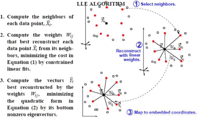
#####################################################################
Here’s how LLE works:
first, for each training instance ![]() , the algorithm identifies its k closest neighbors (in the preceding code k = 10)
, the algorithm identifies its k closest neighbors (in the preceding code k = 10) ,
,
then tries to reconstruct ![]() as a linear function of these neighbors. More specifically, it finds the weights
as a linear function of these neighbors. More specifically, it finds the weights ![]() such that the squared distance between
such that the squared distance between ![]() and
and ![]() is as small as possible, assuming
is as small as possible, assuming ![]() if
if ![]() is not one of the k closest neighbors of
is not one of the k closest neighbors of ![]() . Thus the first step of LLE is the constrained optimization problem described in Equation 8-4, where W is the weight matrix containing all the weights
. Thus the first step of LLE is the constrained optimization problem described in Equation 8-4, where W is the weight matrix containing all the weights ![]() . The second constraint simply normalizes the weights for each training instance
. The second constraint simply normalizes the weights for each training instance ![]() .
.
Equation 8-4. LLE step 1: linearly modeling local relationships
After this step, the weight matrix ![]() (containing the weights
(containing the weights  ) encodes the local linear relationships between the training instances.
Now the second step is to map the training instances into a d-dimensional space (where d < n) while preserving these
local relationships as much as possible. If ![]() is the image of
is the image of ![]() in this d-dimensional space, then we want the squared distance between
in this d-dimensional space, then we want the squared distance between ![]() and
and ![]() to be as small as possible. This idea leads to the unconstrained optimization problem described in Equation 8-5. It looks very similar to the first step, but instead of keeping the instances fixed and finding the optimal weights, we are doing the reverse: keeping the weights fixed and finding the optimal position of the instances’ images in the low dimensional space. Note that Z is the matrix containing all
to be as small as possible. This idea leads to the unconstrained optimization problem described in Equation 8-5. It looks very similar to the first step, but instead of keeping the instances fixed and finding the optimal weights, we are doing the reverse: keeping the weights fixed and finding the optimal position of the instances’ images in the low dimensional space. Note that Z is the matrix containing all ![]() .
.
Scikit-Learn’s LLE implementation has the following computational complexity:O( mlog(m) nlog(k) ) for finding the k nearest neighbors, ![]() for optimizing the weights, and
for optimizing the weights, and ![]() for constructing the low-dimensional representations. Unfortunately, the
for constructing the low-dimensional representations. Unfortunately, the ![]() in the last term makes this algorithm scale poorly to very large datasets.
in the last term makes this algorithm scale poorly to very large datasets.
Other Dimensionality Reduction Techniques
There are many other dimensionality reduction techniques, several of which are available in Scikit-Learn. Here are some of the most popular:
- Multidimensional Scaling (MDS)多维缩放 reduces dimensionality while trying to preserve the distances between the instances (see Figure 8-13).
- Isomap creates a graph by connecting each instance to its nearest neighbors, then reduces dimensionality while trying to preserve the geodesic distances测地线的 between the instances.
- t-Distributed Stochastic Neighbor Embedding (t-SNE) t-分布随机邻域嵌入reduces dimensionality while trying to keep similar instances close and dissimilar instances apart. It is mostly used for visualization, in particular to visualize clusters of instances in high-dimensional space (e.g., to visualize the MNIST images in 2D).
- Linear Discriminant Analysis (LDA) is actually a classification algorithm, but during training it learns the most discriminative区别的 axes between the classes, and these axes can then be used to define a hyperplane onto which to project the data. The benefit is that the projection will keep classes as far apart as possible, so LDA is a good technique to reduce dimensionality before running another classification algorithm such as an SVM classifier.
from sklearn.manifold import MDS

mds = MDS( n_components=2, random_state=42)
X_reduced_mds = mds.fit_transform(X)
# X_reduced_mds.shape #(1000, 2)
from sklearn.manifold import Isomap isomap = Isomap(n_components=2) X_reduced_isomap = isomap.fit_transform(X)from sklearn.manifold import TSNE tsne = TSNE(n_components=2, random_state=42) X_reduced_tsne = tsne.fit_transform(X)from sklearn.discriminant_analysis import LinearDiscriminantAnalysis lda = LinearDiscriminantAnalysis(n_components=2) X_mnist = mnist["data"] y_mnist = mnist["target"] lda.fit(X_mnist, y_mnist) X_reduced_lda = lda.transform(X_mnist) # X_reduced_lda.shape # (70000, 2)titles = ["MDS", "Isomap", "t-SNE"] plt.figure(figsize=(15,4)) for subplot, title, X_reduced in zip((131,132,133), titles, (X_reduced_mds, X_reduced_isomap, X_reduced_tsne)): plt.subplot(subplot) plt.title(title, fontsize=14) #first component #second component plt.scatter(X_reduced[:,0], X_reduced[:,1], c=t, cmap=plt.cm.hot) plt.xlabel("$z_1$", fontsize=18) if( subplot==131): plt.ylabel("$z_2$", fontsize=18, rotation=0) plt.grid(True) plt.show()Figure 8-13. Reducing the Swiss roll to 2D using various techniques

Exercises
https://blog.csdn.net/Linli522362242/article/details/105722461


