机器学习第一周

机器学习第一周

K-近邻算法
算法的核心——采用测量不同特征值之间的距离方法进行分类

• k-近邻算法的优缺点
  优点：精度高，对异常值不敏感，无数据输入假定
  缺点：计算复杂度高，空间复杂度高
• 适应的数据类型：数值型，标称型

使用KNN算法的基本思路（本次学习采用的相关步骤）——

注：对于距离的计算过程中，其实存在多种含义上的距离，目前采用的是欧式距离，对于不同的问题可以拓展到不同的距离上去——曼哈顿距离，切比雪夫距离，马氏距离，巴氏距离，汉明距离，皮尔逊距离，信息熵

使用kNN算法的相关步骤——
1）收集数据 2）准备数据 3）分析数据 4）训练算法 5)测试算法 6）使用算法
首先是要创建数据集，并且对于数据集中的数据进行相关的分类（通过计算距离来确定前k个元素的主要分类），代码如下——

import numpy as np
import operator
def createDataSet():
    group = np.array([[1.0, 1.1], [1.0, 1.0], [0, 0], [0, 0.1]])
    labels = ['A', 'A', 'B', 'B']
    return group, labels
def classify0(inX, dataSet, labels, k):   ##k为我们所要求的k个元素的范围
    dataSetSize = dataSet.shape[0]
    diffMat = np.tile(inX, (dataSetSize, 1)) - dataSet
    sqDiffMat = diffMat**2
    sqDistances = sqDiffMat.sum(axis=1)
    distances = sqDistances**0.5
    sortedDistIndicies = distances.argsort()
    classCount = {}
    for i in range(k):
        voteIlabel = labels[sortedDistIndicies[i]]
        classCount[voteIlabel] = classCount.get(voteIlabel, 0) + 1
    sortedClassCount = sorted(classCount.items(), key=operator.itemgetter(1), reverse=True)
    return sortedClassCount[0][0]

进行试验之后，可以得到我们所要求的结果——

接着，我们对书中的实例进行操作（海伦约会配对）——
首先是分析数据，要对文本进行相关的处理（转换成为Numpy的形式），代码如下——

def file2matrix(filename):
    love_dictionary = {'largeDoses':3, 'smallDoses':2, 'didntLike':1}
    fr = open(filename)
    arrayOLines = fr.readlines()
    numberOfLines = len(arrayOLines)            #get the number of lines in the file
    returnMat = np.zeros((numberOfLines, 3))        #prepare matrix to return
    classLabelVector = []                       #prepare labels return
    index = 0
    for line in arrayOLines:
        line = line.strip()
        listFromLine = line.split('\t')
        returnMat[index, :] = listFromLine[0:3]
        if(listFromLine[-1].isdigit()):
            classLabelVector.append(int(listFromLine[-1]))
        else:
            classLabelVector.append(love_dictionary.get(listFromLine[-1]))
        index += 1
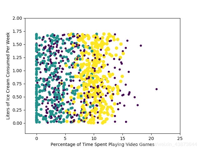
    return returnMat, classLabelVector

采用matplotlib对该数据进行散点图描绘，可以得到以下的结果——

紧接着需要对这些数据进行归一化处理，实现准备数据的过程，方便后面的距离计算——

def autoNorm(dataSet):
    minVals = dataSet.min(0)
    maxVals = dataSet.max(0)
    ranges = maxVals - minVals
    normDataSet = np.zeros(np.shape(dataSet))
    m = dataSet.shape[0]
    normDataSet = dataSet - np.tile(minVals, (m, 1))
    normDataSet = normDataSet/np.tile(ranges, (m, 1))   #element wise divide
    return normDataSet, ranges, minVals

然后是测试算法——

def datingClassTest():
    hoRatio = 0.50      #hold out 10%
    datingDataMat, datingLabels = file2matrix('datingTestSet2.txt')       #load data setfrom file
    normMat, ranges, minVals = autoNorm(datingDataMat)
    m = normMat.shape[0]
    numTestVecs = int(m*hoRatio)
    errorCount = 0.0
    for i in range(numTestVecs):
        classifierResult = classify0(normMat[i, :], normMat[numTestVecs:m, :], datingLabels[numTestVecs:m], 3)
        print("the classifier came back with: %d, the real answer is: %d" % (classifierResult, datingLabels[i]))
        if (classifierResult != datingLabels[i]): errorCount += 1.0
    print("the total error rate is: %f" % (errorCount / float(numTestVecs)))
    print(errorCount)

通过测试可以发现错误率为2.4%
进入下一步，使用算法——

def classifyPerson():
    resultList = ['not at all', 'in small doses', 'in large doses']
    percentTats = float(input(\
                                  "percentage of time spent playing video games?"))
    ffMiles = float(input("frequent flier miles earned per year?"))
    iceCream = float(input("liters of ice cream consumed per year?"))
    datingDataMat, datingLabels = file2matrix('datingTestSet2.txt')
    normMat, ranges, minVals = autoNorm(datingDataMat)
    inArr = np.array([ffMiles, percentTats, iceCream, ])
    classifierResult = classify0((inArr - \
                                  minVals)/ranges, normMat, datingLabels, 3)
    print("You will probably like this person: %s" % resultList[classifierResult - 1])

决策树

• 决策树的优缺点——
  优点：计算复杂度不高，输出结果易于理解，对中间值的缺失不敏感，可以处理不相关的特征数据；其数据形非常容易理解。
  缺点：可能会产生过度匹配问题。
• 适用的数据类型：数值型，标称型（意味着最后的数据必须是离散形式）

构建决策树的基本思路（本次学习中采用的相关步骤）——

关于ID3算法基本简介——
ID3算法是一种贪心算法，起源于概念学习系统，以信息熵的下降速度作为选取测试属性的标准——在每个节点选取“尚未”被用来划分的具有最高信息增益的属性作为划分标准。
算法的核心是信息熵——信息增益高的属性是好属性，每次划分选取信息增益最高的属性作为划分标准，重复该过程，可以实现完美分类训练样例的决策树

关于信息论的一些基本概念——
a.对于信息量的定义——信息Xi的信息量定义为l(Xi)=–log2(p(Xi))
b.对于熵的定义（信息量的期望值）——H=-∑p(Xi)*log2(p(Xi))

由于最开始寻找划分数据集的特征是按照对于熵的比较进行的，那么最开始编写计算香农熵的函数，代码如下——

from math import log
def calcShannonEnt(dataSet):
    numEntries=len(dataSet)
    labelCounts={}
    for featVec in dataSet:
        currentLabel=featVec[-1]
        if currentLabel not in labelCounts.keys(): labelCounts[currentLabel] = 0
        labelCounts[currentLabel] += 1
    shannonEnt = 0.0
    print(labelCounts)
    for key in labelCounts:
        prob = float(labelCounts[key]) / numEntries
        shannonEnt -= prob * log(prob, 2)  # log base 2
    return shannonEnt

通过计算香农熵之后，可以对于信息数据的无序程度进行度量，那么需要对数据进行划分，划分一次计算一次香农熵，并且选出最佳的香农熵对应的划分特征，代码如下——

def splitDataSet(dataSet, axis, value):
    retDataSet = []
    for featVec in dataSet:
        if featVec[axis] == value:
            reducedFeatVec = featVec[:axis]     #chop out axis used for splitting
            reducedFeatVec.extend(featVec[axis+1:])
            retDataSet.append(reducedFeatVec)
    return retDataSet


def chooseBestFeatureToSplit(dataSet):
    numFeatures = len(dataSet[0]) - 1      #the last column is used for the labels
    baseEntropy = calcShannonEnt(dataSet)
    bestInfoGain = 0.0; bestFeature = -1
    for i in range(numFeatures):        #iterate over all the features
        featList = [example[i] for example in dataSet]#create a list of all the examples of this feature
        uniqueVals = set(featList)       #get a set of unique values
        newEntropy = 0.0
        for value in uniqueVals:
            subDataSet = splitDataSet(dataSet, i, value)
            prob = len(subDataSet)/float(len(dataSet))
            newEntropy += prob * calcShannonEnt(subDataSet)
        infoGain = baseEntropy - newEntropy     #calculate the info gain; ie reduction in entropy
        if (infoGain > bestInfoGain):       #compare this to the best gain so far
            bestInfoGain = infoGain         #if better than current best, set to best
            bestFeature = i
    return bestFeature                      #returns an integer

在明确已知的特征之后，我们开始根据这些特征创建相应的树，采用递归的方式。代码如下——

def majorityCnt(classList):
    classCount={}
    for vote in classList:
        if vote not in classCount.keys(): classCount[vote] = 0
        classCount[vote] += 1
    sortedClassCount = sorted(classCount.items(), key=operator.itemgetter(1), reverse=True)
    return sortedClassCount[0][0]

def createTree(dataSet, labels):
    classList = [example[-1] for example in dataSet]
    if classList.count(classList[0]) == len(classList):
        return classList[0]#stop splitting when all of the classes are equal
    if len(dataSet[0]) == 1: #stop splitting when there are no more features in dataSet
        return majorityCnt(classList)
    bestFeat = chooseBestFeatureToSplit(dataSet)
    bestFeatLabel = labels[bestFeat]
    myTree = {bestFeatLabel:{}}
    del(labels[bestFeat])
    featValues = [example[bestFeat] for example in dataSet]
    uniqueVals = set(featValues)
    for value in uniqueVals:
        subLabels = labels[:]       #copy all of labels, so trees don't mess up existing labels
        myTree[bestFeatLabel][value] = createTree(splitDataSet(dataSet, bestFeat, value), subLabels)
    return myTree

目前来看，基本上完成了关于树的创建，但是为了更加直观的将树的形式展现出来，采用了matplotlib的模块对创建的树进行表达，即以图像形式表达最后的决策树。代码如下——

import matplotlib.pyplot as plt
decisionNode = dict(boxstyle="sawtooth", fc="0.8")
leafNode = dict(boxstyle="round4", fc="0.8")
arrow_args = dict(arrowstyle="<-")

def getNumLeafs(myTree):
    numLeafs = 0
    firstStr = list(myTree)[0]
    secondDict = myTree[firstStr]
    for key in secondDict.keys():
        if type(secondDict[key]).__name__ == 'dict':#test to see if the nodes are dictonaires, if not they are leaf nodes
            numLeafs += getNumLeafs(secondDict[key])
        else: numLeafs += 1
    return numLeafs
def getTreeDepth(myTree):
    maxDepth = 0
    firstStr = list(myTree)[0]
    secondDict = myTree[firstStr]
    for key in secondDict.keys():
        if type(secondDict[key]).__name__ == 'dict':#test to see if the nodes are dictonaires, if not they are leaf nodes
            thisDepth = 1 + getTreeDepth(secondDict[key])
        else: thisDepth = 1
        if thisDepth > maxDepth: maxDepth = thisDepth
    return maxDepth
def plotNode(nodeTxt, centerPt, parentPt, nodeType):
    createPlot.ax1.annotate(nodeTxt, xy=parentPt, xycoords='axes fraction',
                            xytext=centerPt, textcoords='axes fraction',
                            va="center", ha="center", bbox=nodeType, arrowprops=arrow_args)
def plotMidText(cntrPt, parentPt, txtString):
    xMid = (parentPt[0]-cntrPt[0])/2.0 + cntrPt[0]
    yMid = (parentPt[1]-cntrPt[1])/2.0 + cntrPt[1]
    createPlot.ax1.text(xMid, yMid, txtString, va="center", ha="center", rotation=30)
def plotTree(myTree, parentPt, nodeTxt):#if the first key tells you what feat was split on
    numLeafs = getNumLeafs(myTree)  #this determines the x width of this tree
    depth = getTreeDepth(myTree)
    firstStr = list(myTree)[0]     #the text label for this node should be this
    cntrPt = (plotTree.xOff + (1.0 + float(numLeafs))/2.0/plotTree.totalW, plotTree.yOff)
    plotMidText(cntrPt, parentPt, nodeTxt)
    plotNode(firstStr, cntrPt, parentPt, decisionNode)
    secondDict = myTree[firstStr]
    plotTree.yOff = plotTree.yOff - 1.0/plotTree.totalD
    for key in secondDict.keys():
        if type(secondDict[key]).__name__ == 'dict':#test to see if the nodes are dictonaires, if not they are leaf nodes
            plotTree(secondDict[key], cntrPt, str(key))        #recursion
        else:   #it's a leaf node print the leaf node
            plotTree.xOff = plotTree.xOff + 1.0/plotTree.totalW
            plotNode(secondDict[key], (plotTree.xOff, plotTree.yOff), cntrPt, leafNode)
            plotMidText((plotTree.xOff, plotTree.yOff), cntrPt, str(key))
    plotTree.yOff = plotTree.yOff + 1.0/plotTree.totalD
def createPlot(inTree):
    fig = plt.figure(1, facecolor='white')
    fig.clf()
    axprops = dict(xticks=[], yticks=[])
    createPlot.ax1 = plt.subplot(111, frameon=False, **axprops)    #no ticks
    #createPlot.ax1 = plt.subplot(111, frameon=False) #ticks for demo puropses
    plotTree.totalW = float(getNumLeafs(inTree))
    plotTree.totalD = float(getTreeDepth(inTree))
    plotTree.xOff = -0.5/plotTree.totalW; plotTree.yOff = 1.0
    plotTree(inTree, (0.5, 1.0), '')
    plt.show()
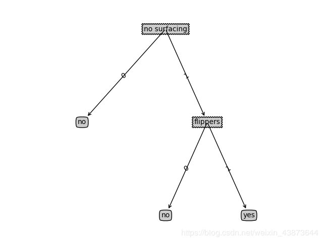
def retrieveTree(i):
    listOfTrees = [{'no surfacing': {0: 'no', 1: {'flippers': {0: 'no', 1: 'yes'}}}},
                   {'no surfacing': {0: 'no', 1: {'flippers': {0: {'head': {0: 'no', 1: 'yes'}}, 1: 'no'}}}}
                  ]
    return listOfTrees[i]

经过代码推演，得到结果如下：

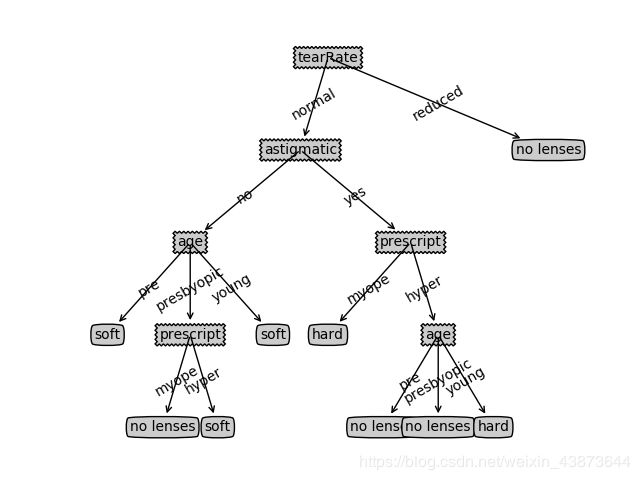
紧接着，对于书中给出的实例进行了演练（预测隐形眼镜类型），得到的结果如下——