小白机器学习进阶之路2——线性回归

小白机器学习进阶之路2——线性回归

第一周学习了线性回归模型。下面以第一周的作业为例总结一下。
解决线性回归

1. gradient descent
2. normal equation
   问题：
   给出数据
   
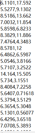
   用代码实现线性回归
   1.gradient descent method

import numpy as np
import pandas as pd
import matplotlib.pyplot as plt

首先调入包 numpy（关于矩阵）pandas（数据处理）matplotlib.pyplot（python中的画图）

path =  'ex1data1.txt'
data = pd.read_csv(path, header=None, names=['Population', 'Profit'])
data.head()  #预览数据

注意，这里要把数据的文本文档和代码的文档放在一个文件夹下，否则就要使用绝对路径。

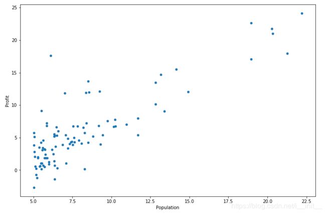
data.plot(kind='scatter', x='Population', y='Profit', figsize=(12,8))
plt.show()

画散点图

构建代价函数（差的平方和）

def computeCost(X, y, theta):
    error = np.power(((X*theta.T)-y),2)
    errorSquareSum = np.sum(error)
    return errorSquareSum/(2*len(X))

data.insert(0, 'Ones', 1)

在矩阵X下插入第一列全为一，保证将X*theta.T-y转换成误差，方便写公式。

X = np.matrix(X.values)
y = np.matrix(y.values)
# your code here  (appro ~ 1 lines)
theta = np.matrix(np.array([0,0]))

将X和y和theta转换成np能够操作的矩阵并初始化theta的值。
由于单变量，theta有两列

现在X是972 的矩阵，第一列全为1，第二列是自变量的值。
theta是12 的矩阵，第一列是θ0，第二列是θ1。
y是97*1的矩阵，是因变量的值。

def gradientDescent(X, y, theta, alpha, iters):
    temp = np.matrix(np.zeros(theta.shape))
    #定义一个theta形状的零矩阵
    parameters = int(theta.ravel().shape[1])
    #定义一个变量，表示theta的个数。
    #ravel函数将矩阵变为一维，shape[1]代表了矩阵的列数（即theta的个数）
    cost = np.zeros(iters)
    
    for i in range(iters):
       
        error = (X*theta.T)-y
        for j in range(parameters):
            
            term = np.multiply(error, X[:,j])#计算两矩阵(hθ(x)-y)x
            temp[0,j] = theta[0,j] - ((alpha / len(X)) * np.sum(term))
            
        
        cost[i] = computeCost(X,y,theta)
        theta = temp
    return theta, cost

定义gradient descent 函数。需要的参数为自变量因变量theta迭代速率和迭代次数。
alpha = 0.01
iters = 1000
初始化迭代速率和次数

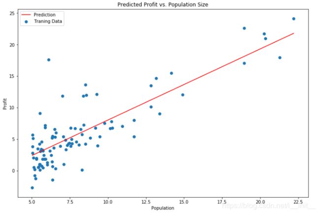
运行之后的结果：

画图

代价函数最小化过程的变化图

总结：
用到的函数
表格形式读取数据：pd.read_csv(path,header,names = [])
画图：plot方法 .plot(kind =’’, x = ‘’, y = ‘’,figsize = ())
plt.show()
iloc方法，抽取数据
关于矩阵：
np.power()对矩阵中的数值进行平方，不改变形状
np.sum() 求和
shape[0] shape[1]代表矩阵的行数和列数
np.zeros() 创建零矩阵
np.multiply() 矩阵的乘法
np.linspace() 在一定范围内抽取样本

2.normal equation method
公式θ = （XTX）-1XTy

normal equation 方法没有仔细做，就略过吧

#作业源
吴恩达机器学习