机器学习之非监督学习——(猫狗识别案例/搭建卷积神经网络)
非监督学习
监督学习的存在它的弊端,例如对我们人类还无法分辨和归类的事物,监督学习就无法完成,所以为了弥补这个缺陷,下面我们看一下新非监督学习,它可以让计算机学会进行更加复杂的分类。
分析过程
非监督学习的构建一般由三个部分组成,数据的预处理,神经网络的搭建,然后进行训练测试,训练测试生成数据集和模型,最后倒入已知数据,让计算机对我们输入的数据进行分类。
项目案例:
猫狗识别
知识点:
1、数据的预处理
2、搭建神经网络
3、模型的训练与储存
项目分步分析:
第一步:创建六个文件夹

1、log文件夹,用于存放丢失数据和数据误差
2、modelsave文件夹用于存放训练好的模型
3、train_image文件夹用于,存放猫狗的图片,这些图片是作为训练模型的数据
4、train.py 用于进行数据的预处理和模型的搭建
5、model.py 搭建神经网络
6、test.py 测试搭建好的模型,用于猫狗识别
第二步:train_image文件内容
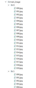
在train_image文件夹中穿件名为0的文件夹,用于存放猫的图片(数据),然后创建名为1的文件夹,用于存放狗的数据。
创建好0和1的文件之后,分别放入 猫和狗的图片。
第三步:train.py 文件第一部分的内容,对数据进行预处理,数据的预处理分为连个步骤,第一步是获取数据并生成标签集,第二不是将数据进行分批处理。
		#导入tensorflow
		import tensorflow as tf
		#创建函数获取train_image中的文件,生成标签集合
		def get_files(file_path):
	 #两个文件,一个是用于存放图片路径,一个是用于对图片标记
	   class_train = []
	   label_train = []
	   #根据路径将图片遍历出来
	   for train_class in os.listdir(file_path):
	      #pic_name is the train image name
	      for pic_name in os.listdir(file_path + train_class):
		 #添加入前面创建好的列表当中
	         class_train.append(file_path + train_class + '/' + pic_name)
	         #train_class is 0,1,2,3,4....
	         label_train.append(train_class)
	   #将trainimage和trainlabel合并到二维数组(2,n)
	   temp = np.array([class_train, label_train])
	   #进行数据降维
	   temp = temp.transpose()
	   np.random.shuffle(temp)
	#获取降维后的数据
	   image_list = list(temp[:,0])
	   label_list = list(temp[:,1])
	   label_list = [int(i) for i in label_list]
	   return image_list, label_list

	def get_batches(image, label, resize_w, resize_h, batch_size, capacity):
	   #用TensorFlow进行数据字符的提取
	   image = tf.cast(image, tf.string)
	   #用TensorFlow进行特殊字符的标记,为64位
	   label = tf.cast(label, tf.int64)
	#让图片和标记形成队列
	   queue = tf.train.slice_input_producer([image, label])
	   label = queue[1]
	   image_temp = tf.read_file(queue[0])
	   image = tf.image.decode_jpeg(image_temp, channels = 3)
	   #宠幸标记图片型号
	   image = tf.image.resize_image_with_crop_or_pad(image, resize_w, resize_h)

	   image = tf.image.per_image_standardization(image)

	   image_batch, label_batch = tf.train.batch([image, label], batch_size = batch_size,
	      num_threads = 64,
	      capacity = capacity)
	   images_batch = tf.cast(image_batch, tf.float32)
	   labels_batch = tf.reshape(label_batch, [batch_size])
	   return images_batch, labels_batch
model.py 设计神经网络,神经网络的结构
conv1 卷积层 1
pooling1_lrn 池化层 1
conv2 卷积层 2
pooling2_lrn 池化层 2
local3 全连接层 1
local4 全连接层 2
softmax 全连接层 3
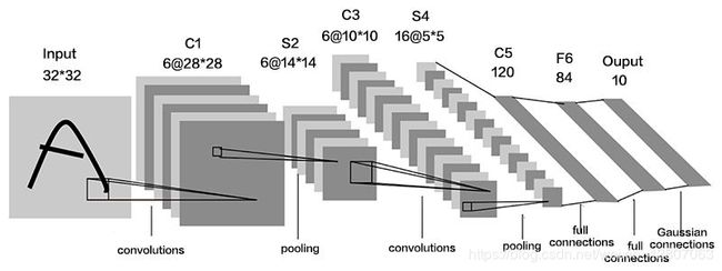
1、以上是网络神经的结构,我们来开始搭建,代码如下:
#导入tensorflow
Im#port tensorflow as tf
#对数据分批处理
def inference(images, batch_size, n_classes):
卷积层1 conv1
with tf.variable_scope('conv1') as scope:
    weights = tf.Variable(tf.truncated_normal(shape=[3, 3, 3, 64], stddev=1.0, dtype=tf.float32),
                          name='weights', dtype=tf.float32)

    biases = tf.Variable(tf.constant(value=0.1, dtype=tf.float32, shape=[64]),
                         name='biases', dtype=tf.float32)

    conv = tf.nn.conv2d(images, weights, strides=[1, 1, 1, 1], padding='SAME')
    pre_activation = tf.nn.bias_add(conv, biases)
    conv1 = tf.nn.relu(pre_activation, name=scope.name)
池化层 1 pooling1
with tf.variable_scope('pooling1_lrn') as scope:
    pool1 = tf.nn.max_pool(conv1, ksize=[1, 3, 3, 1], strides=[1, 2, 2, 1], padding='SAME', name='pooling1')
    norm1 = tf.nn.lrn(pool1, depth_radius=4, bias=1.0, alpha=0.001 / 9.0, beta=0.75, name='norm1')
卷积层2 conv2
with tf.variable_scope('conv2') as scope:
    weights = tf.Variable(tf.truncated_normal(shape=[3, 3, 64, 16], stddev=0.1, dtype=tf.float32),
                          name='weights', dtype=tf.float32)

    biases = tf.Variable(tf.constant(value=0.1, dtype=tf.float32, shape=[16]),
                         name='biases', dtype=tf.float32)

    conv = tf.nn.conv2d(norm1, weights, strides=[1, 1, 1, 1], padding='SAME')
    pre_activation = tf.nn.bias_add(conv, biases)
    conv2 = tf.nn.relu(pre_activation, name='conv2')
池化层 2 pooling2
with tf.variable_scope('pooling2_lrn') as scope:
    norm2 = tf.nn.lrn(conv2, depth_radius=4, bias=1.0, alpha=0.001 / 9.0, beta=0.75, name='norm2')
    pool2 = tf.nn.max_pool(norm2, ksize=[1, 3, 3, 1], strides=[1, 1, 1, 1], padding='SAME', name='pooling2')
全连接层1 local3
with tf.variable_scope('local3') as scope:
    reshape = tf.reshape(pool2, shape=[batch_size, -1])
    dim = reshape.get_shape()[1].value
    weights = tf.Variable(tf.truncated_normal(shape=[dim, 128], stddev=0.005, dtype=tf.float32),
                          name='weights', dtype=tf.float32)

    biases = tf.Variable(tf.constant(value=0.1, dtype=tf.float32, shape=[128]),
                         name='biases', dtype=tf.float32)

    local3 = tf.nn.relu(tf.matmul(reshape, weights) + biases, name=scope.name)
全连接层2 local4
with tf.variable_scope('local4') as scope:
    weights = tf.Variable(tf.truncated_normal(shape=[128, 128], stddev=0.005, dtype=tf.float32),
                          name='weights', dtype=tf.float32)

    biases = tf.Variable(tf.constant(value=0.1, dtype=tf.float32, shape=[128]),
                         name='biases', dtype=tf.float32)

    local4 = tf.nn.relu(tf.matmul(local3, weights) + biases, name='local4')
全连接层 3 softmax
with tf.variable_scope('softmax_linear') as scope:
    weights = tf.Variable(tf.truncated_normal(shape=[128, n_classes], stddev=0.005, dtype=tf.float32),
                          name='softmax_linear', dtype=tf.float32)

    biases = tf.Variable(tf.constant(value=0.1, dtype=tf.float32, shape=[n_classes]),
                         name='biases', dtype=tf.float32)

    softmax_linear = tf.add(tf.matmul(local4, weights), biases, name='softmax_linear')

return softmax_linear
剔除无用数据并获得loss
def losses(logits, labels):
    with tf.variable_scope('loss') as scope:
        cross_entropy = tf.nn.sparse_softmax_cross_entropy_with_logits(logits=logits, labels=labels,
                                                                       name='xentropy_per_example')
        loss = tf.reduce_mean(cross_entropy, name='loss')
        tf.summary.scalar(scope.name + '/loss', loss)
    return loss
#进行数据优化
def trainning(loss, learning_rate):
    with tf.name_scope('optimizer'):
        optimizer = tf.train.AdamOptimizer(learning_rate=learning_rate)
        global_step = tf.Variable(0, name='global_step', trainable=False)
        train_op = optimizer.minimize(loss, global_step=global_step)
    return train_op


#显示精确度
def evaluation(logits, labels):
    with tf.variable_scope('accuracy') as scope:
        correct = tf.nn.in_top_k(logits, labels, 1)
        correct = tf.cast(correct, tf.float16)
        accuracy = tf.reduce_mean(correct)
        tf.summary.scalar(scope.name + '/accuracy', accuracy)
    return accuracy
第四步:train.py 文件第二部分的内容:训练数据,并将训练的模型存储
#导入所需要的功能库
import matplotlib.pyplot as plt
import numpy as np
import os
import PIL.Image as Image
import model

#loss数据文件存放路径
LOG_DIR = './log'
#生个数据模型存放路径
CHECK_POINT_DIR = './modelsave'
数据的预处理
下面是对特殊数据进行解释说明
N_CLASSES = 2 # 2个输出神经元,[1,0] 或者 [0,1]猫和狗的概率
IMG_W = 64 # 重新定义图片的大小,图片如果过大则训练比较慢
IMG_H = 64
BATCH_SIZE = 10 #每批数据的大小
CAPACITY = 20
MAX_STEP = 15000 # 训练的步数,应当 >= 10000
learning_rate = 0.0001 # 学习率,建议刚开始的 learning_rate <= 0.0001
#训练程序
def run_training():
# 数据集
train_dir='./train_image/'
# 获取图片和标签集
train,train_label = get_files(train_dir)
# 生成批次
train_batch, train_label_batch = get_batches(train, train_label, IMG_W, IMG_H, BATCH_SIZE, CAPACITY)
# 进入模型
train_logits = model.inference(train_batch, BATCH_SIZE, N_CLASSES)
# 获取 loss
train_loss = model.losses(train_logits, train_label_batch)
# 训练
train_op = model.trainning(train_loss, learning_rate)
# 获取准确率
train_acc = model.evaluation(train_logits, train_label_batch)
# 合并 summary
summary_op = tf.summary.merge_all()
sess = tf.Session()
# 保存summary
train_writer = tf.summary.FileWriter(LOG_DIR, sess.graph)
saver = tf.train.Saver()
sess.run(tf.global_variables_initializer())
coord = tf.train.Coordinator()
threads = tf.train.start_queue_runners(sess=sess, coord=coord)
try:
for step in np.arange(1000):
if coord.should_stop():
break
_, tra_loss, tra_acc = sess.run([train_op, train_loss, train_acc])
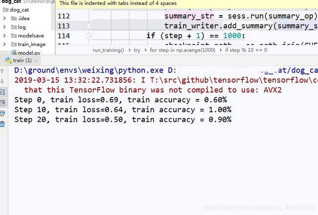
if step % 10 == 0:
print('Step %d, train loss=%.2f, train accuracy = %.2f%%' %(step, tra_loss, tra_acc))
summary_str = sess.run(summary_op)-
train_writer.add_summary(summary_str, step)
# 每隔2000步保存一下模型,模型保存在 checkpoint_path 中
if (step + 1) == 1000:
checkpoint_path = os.path.join(CHECK_POINT_DIR, 'model_ckpt')
saver.save(sess, checkpoint_path, global_step=step)
except tf.errors.OutOfRangeError:
print ('Done training')
finally:
coord.request_stop()
coord.join(threads)
if __name__=="__main__":
run_training()
第五步:test.py 测试搭建好的模型,进行猫够识别,在网上随便下载一只猫或者狗,导入模型,进行识别,最终让电脑告诉我们我们放进去的到底是猫还是狗:
先导入要使用的功能库
#用于图形处理
from PIL import Image
import numpy as np
import tensorflow as tf
#用于数据可视化
import matplotlib.pyplot as plt
#导入神经网络
import model
#模型存放路径
CHECK_POINT_DIR = './modelsave'
#进行图像识别
def evaluate_one_image(image_array):
with tf.Graph().as_default():
BATCH_SIZE = 1 # 因为只读取一副图片 所以batch 设置为1
N_CLASSES = 2 # 2个输出神经元,[1,0] 或者 [0,1]猫和狗的概率
# 转化图片格式
image = tf.cast(image_array, tf.float32)
# 图片标准化
image = tf.image.per_image_standardization(image)
# 图片原来是三维的 [64,64,3] 重新定义图片形状 改为一个4D 四维的 tensor
image = tf.reshape(image, [1, 64,64,3])
logit = model.inference(image, BATCH_SIZE, N_CLASSES)
# 因为 inference 的返回没有用激活函数,所以在这里对结果用softmax 激活
logit = tf.nn.softmax(logit)
# 定义saver
saver = tf.train.Saver()
with tf.Session() as sess:
# print ('Reading checkpoints...')
print ('从指定的路径中加载模型。。。。')
# 将模型加载到sess 中
ckpt = tf.train.get_checkpoint_state(CHECK_POINT_DIR)
if ckpt and ckpt.model_checkpoint_path:
global_step = ckpt.model_checkpoint_path.split('/')[-1].split('-')[-1]
saver.restore(sess, ckpt.model_checkpoint_path)
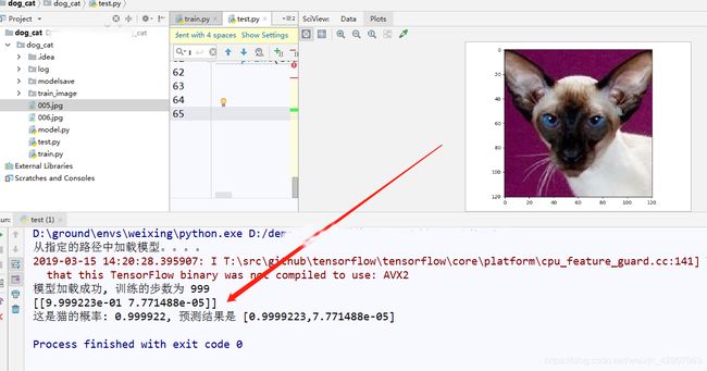
print('模型加载成功, 训练的步数为 %s' %global_step)
else:
print ('模型加载失败,,,文件没有找到')
prediction = sess.run(logit)
# 获取输出结果中最大概率的索引
max_index = np.argmax(prediction)
print (prediction)
if max_index == 0:
result = ('这是猫的概率: %.6f, 预测结果是 [%s]' %(prediction[:,0],','.join(str(i) for i in prediction[0])))
else:
result = ('这是狗的概率: %.6f, 预测结果是 [%s]' %(prediction[:,1],','.join(str(i) for i in prediction[0])))
return result
if __name__ == '__main__':
#打开要识别的图片
image = Image.open('./005.jpg')
# 显示出来
plt.imshow(image)
plt.show()
image = image.resize([64,64])
image = np.array(image)
print(evaluate_one_image(image))
将下面这张长得很像狗的猫咪图片命名为005.jpg,导入进去进行测试
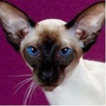
测试结果如下:
然后将下面这张长得很像猫的狗狗图片命名为006.jpg,导入进去进行测试
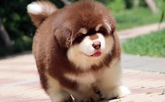
测试结果如下:

总结:
在这个案例中我们充分了解到非监督学习的优点,那就是对比监督学习使用起来十分的灵活,但是相对监督学习对输入和输出的数据都有一个提前预知不同,非监督学习的数据输出是未知和不可控的。这里我们还学习了神经网路的组成和搭建,通过神经网络,我们可以让计算机更像人类一样去识别未知的事物,更好的帮助人类对复杂的事情进行分类,比如博主主题分类,各种主题五花八门,人类分类起来很困难,这就可以用非监督学习,让算计帮助我们进行分类,从这里可以看出非监督学习是致力于解决较为复杂的识别的事物的。