3D Human Pose Estimation from Monocular Images with Deep Convolutional Neural Network（2014）

Deep network for 3D pose estimation（2014）

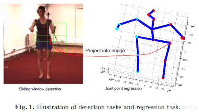
本文提出两种策略去训练deep convolutional neural network以进行3D pose estimation。网络框架包含两个任务：（1）a joint point regression task;（2）joint point detection tasks。两个任务的输入都是包含human subjects的bounding box图片。回归任务是估计关节点相对于根关节点的位置。We define a set of detection tasks,each of which is associated with one joint point and one local window.The aim of each detection task is to clssify whether one local window contains the specific joint or not.

###1. Notation
$$J_i=(J_{i,x},j_{i,y},J_{i,z})$$——the location of the i-th joint in the camera coordinate system.
P——人体的结构化骨骼模型，即关节之间的父子关系。
P(i)——the parent joint of the i-th joint.
根关节的父关节是本身。

2. Joint point regression task

目标：关节点相对于父关节的位置
$$R_i=J_i-J_{P(i)}(1)$$
——$R_i和\widehat{R_i}分别是i-th个关节点的ground-truth和估计的相对位置$
原因：

（1）父子关节点之间的相对位置关系更容易获取
（2）由于人体的对称性，不同关节点之间可以分享信息；如左臂和右臂有相同的长度
（3）在给定对称部分的前提下，易于推断出遮挡关节点的位置

损失函数：
$$E_r(R_i,\widehat{R_i})=||R_i-\widehat{R_i}|{|}_2^2(2)$$
——$R_i和\widehat{R_i}分别是i-th个关节点的ground-truth和估计的相对位置$

3. Joint point detection task

Inspired by[25],we define a set of detection tasks for each joint i and each window l,where the goal is to predict the indicator variable
$$h_{i,l}=\{\begin{array}{l}1,if{B}_{i}isinsidewindowsl,\\ 0,otherwise,\end{array}(3)$$
——$B_i是输入boundingbox中i-th的关节点的2D图片位置$
$B_i$可以通过将$J_i$映射到图片，计算与与bounding box的相对位置而得到。In this work, we do not consider whether the joints are visible or not, i.e., the indicator variables are calculated regardless if the joint is occluded. The reason for doing this is to train the network to learn features for pose estimation even in the presence of occlusions, which might enable the network to predict valid poses when occlusion occur.
损失函数：
$$E_d({\hat{h}}_{i,l},h_{i,l})=-h_{i,l}log({\hat{h}}_{i,l})-(1-h_{i,l})log(1-{\hat{h}}_{i,l})(4)$$
——最小化ground-truth label$h_{i,l}$和estimated label${\hat{h}}_{i,l}$的cross-entropy
The relationship between the regrssion tasks and detection tasks is illustrated in Figure 1

4. Network architecture and multi-task training

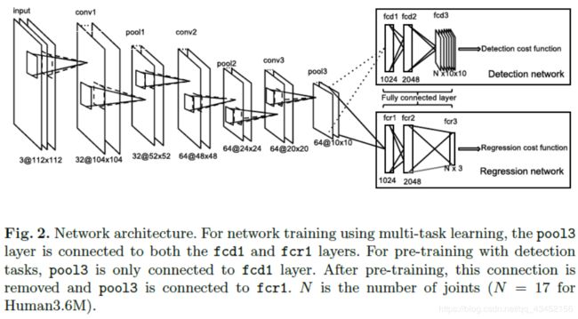
The whole network consists of 9 trainable layers - 3 convolutional layers that are shared by both regression and detecton networks, 3 fully connected layers for the regression network, and 3 fully connected layers for th detection networks.Rectified linear units(ReLu)[30] are used for conv1, conv2, and the first two fully connected layers for both regression and detection networks. We use tanh as the activation function for the last regression normalization layers after conv2,which applies the following function to calculate the output values,
$$f(u_{x,y})=\frac{u_{x,y}}{(1+\frac{\alpha }{|W_x|\cdot |W_y|}{\sum }_{x^{\prime }\in W_x}{\sum }_{y^{\prime }\in W_y}{u}_{x^{\prime },y^{\prime }}^2{)}^{\beta }}(5)$$
——$u_{x,y}$is the value of the previous layer at location$(x,y)$,$(W_x,W_y)$are the neighborhood of locations $(x,y)$,$|W|$represents th number of pixels within the neighborhood,and{$\alpha ,\beta$}are hyper-parameters.
We train the network within a multi-task learning framework. As in [25], we allow features in the lower layers to be shared between the regression and detection tasks during joint training. During the training, the gradients from both networks will be back-propagated to the same shared feature network, i.e., the network with layers from conv1 to pool3. In this case, the shared network tends to learn features that will benefit both tasks. The global cost function for multi-task training is
$${\varphi }_M=\frac{1}{2}\sum _{t=1}^T\sum _{i=1}^N{E}_r(R_i^{(t)},{\hat{R}}_i^t)+\frac{1}{2}\sum _{t=1}^T\sum _{i=1}^N\sum _{l=1}^L{E}_d(h_{i,l}^{(t)},{\hat{h}}_{i,l}^{(t)})(6)$$
——上标$t$是训练样本的索引，$N$是关节点的数目，$T$是训练样本总数

5.Pre-training with the detction task

As an alternative to the multi-task training discussed earlier, another approach is to train the pose regression network using pre-trained weights from the detection network. Firstly we train the detection network alone, i.e., the connections between the pool3 layer and the fcr1 layer are blocked. In this stage, we only minimize the second term in (6). After training the detection tasks, we block the connection between pool3 and fcd1 (thus removing the detection task), and reconnect pool3 to fcr1 layer. Using this strategy, the training for pose regression is initialized using the feature layer weights (conv1-conv3) learned from the detection tasks. Finally, the pose regression is trained using the first term in (6) as the cost function. Note that we do not use the weights of the fully-connected layers of the detectors (fcd1 and fcd2) to initialize fully-connected layers of the regression task (fcr1 and fcr2). The reason is that the target for the detection and regression tasks are quite different, so that the higher-level features used by the detection tasks might not be useful for regression.

6.Training details

For both the multi-task and pre-training approaches, we use back propagation [31] to update the weights during training. In multi-task training, the pool3 layer forwards its values to both fcd1 and fcr1, and receives the average of the gradients from fcd1 and fcr1 when updating the weights. To reduce overfitting, we use “dropout” [32] in fcr1 and fcd1, and set the dropout rate to 0.25. The hyper-parameters for the local response normalization layer are set to $\alpha$ = 0.0025 and $\beta$ = 0.75. More training details can be found in [13].

Experiment

Data augmentation

After obtaining the bounding box of the human subject (provided by the Human3.6M dataset), we resize the bounding box to 128⇥128, such that the aspect ratio of the image is maintained. In order to make the network robust to the selection of the bounding box, in each iteration, a sub-window of size 112⇥112 is randomly selected as the training image (the 2D joint point projections are also adjusted accordingly). Random pixel noise is also added to each input image during training to make the network robust to small perturbations of pixel values. As in [13] we apply PCA on the RGB channels over the whole training samples. In the training stage, we add random noise to all the pixels in each image,
$$\hat{p}=p+[e_1,e_2,e_3]\cdot [g_1{\sqrt{\alpha }}_1,g_2{\sqrt{\alpha }}_2,g_3{\sqrt{\alpha }}_3{]}^T,(7)$$
——$[e_1,e_2,e_3]$and $[{\alpha }_1,{\alpha }_2,{\alpha }_3]$are the eigenvectors and eigenvalues of the $3\times 3$RGB covariance matrix of the triaining set,and $\{g_c{\}}_{c=1}^3$ are each Gaussian distributions with zero mean and variance 0.1.In each iteration,all the pixels within one training sample will share the same random values $\{g_c{\}}_{c=1}^3$.

Evaluation on Human36M

详见原文
Pose predictions are evaluated using the mean per joint position error(MPJPE)[12],
$$MPJPE=\frac{1}{T}\frac{1}{N}\sum _{t=1}^T\sum _{i=1}^N||(J_i^{(t)}-J_{r}oo{t}^{(t)})-({\hat{J}}_i^{(t)}-{\hat{J}}_{r}oo{t}^{(t)})||,(8)$$

Visualization of learned structures

详见原文

Conclusion

（1）采用多任务训练框架：检测和回归
（2）共享低层特征（共享权值）
（3）探讨了DNN如何编码人体结构的依赖性与相关性