动手学深度学习PyTorch版-过拟合欠拟合及其解决方案

过拟合、欠拟合及其解决方案

多项式拟合实验

%matplotlib inline
import torch
import numpy as np
import sys
sys.path.append("/home/kesci/input")
import d2lzh1981 as d2l
print(torch.__version__)

初始化模型参数

n_train, n_test, true_w, true_b = 100, 100, [1.2, -3.4, 5.6], 5
features = torch.randn((n_train + n_test, 1))
poly_features = torch.cat((features, torch.pow(features, 2), torch.pow(features, 3)), 1) 
labels = (true_w[0] * poly_features[:, 0] + true_w[1] * poly_features[:, 1]
          + true_w[2] * poly_features[:, 2] + true_b)
labels += torch.tensor(np.random.normal(0, 0.01, size=labels.size()), dtype=torch.float)

定义训练和测试模型

def semilogy(x_vals, y_vals, x_label, y_label, x2_vals=None, y2_vals=None,
             legend=None, figsize=(3.5, 2.5)):
    # d2l.set_figsize(figsize)
    d2l.plt.xlabel(x_label)
    d2l.plt.ylabel(y_label)
    d2l.plt.semilogy(x_vals, y_vals)
    if x2_vals and y2_vals:
        d2l.plt.semilogy(x2_vals, y2_vals, linestyle=':')
        d2l.plt.legend(legend)
num_epochs, loss = 100, torch.nn.MSELoss()

def fit_and_plot(train_features, test_features, train_labels, test_labels):
    # 初始化网络模型
    net = torch.nn.Linear(train_features.shape[-1], 1)
    # 通过Linear文档可知，pytorch已经将参数初始化了，所以我们这里就不手动初始化了
    
    # 设置批量大小
    batch_size = min(10, train_labels.shape[0])    
    dataset = torch.utils.data.TensorDataset(train_features, train_labels)      # 设置数据集
    train_iter = torch.utils.data.DataLoader(dataset, batch_size, shuffle=True) # 设置获取数据方式
    
    optimizer = torch.optim.SGD(net.parameters(), lr=0.01)                      # 设置优化函数，使用的是随机梯度下降优化
    train_ls, test_ls = [], []
    for _ in range(num_epochs):
        for X, y in train_iter:                                                 # 取一个批量的数据
            l = loss(net(X), y.view(-1, 1))                                     # 输入到网络中计算输出，并和标签比较求得损失函数
            optimizer.zero_grad()                                               # 梯度清零，防止梯度累加干扰优化
            l.backward()                                                        # 求梯度
            optimizer.step()                                                    # 迭代优化函数，进行参数优化
        train_labels = train_labels.view(-1, 1)
        test_labels = test_labels.view(-1, 1)
        train_ls.append(loss(net(train_features), train_labels).item())         # 将训练损失保存到train_ls中
        test_ls.append(loss(net(test_features), test_labels).item())            # 将测试损失保存到test_ls中
    print('final epoch: train loss', train_ls[-1], 'test loss', test_ls[-1])    
    semilogy(range(1, num_epochs + 1), train_ls, 'epochs', 'loss',
             range(1, num_epochs + 1), test_ls, ['train', 'test'])
    print('weight:', net.weight.data,
          '\nbias:', net.bias.data)

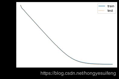
三阶多项式拟合

fit_and_plot(poly_features[:n_train, :], poly_features[n_train:, :], labels[:n_train], labels[n_train:])

final epoch: train loss 0.00011492073099361733 test loss 0.00010899170592892915
weight: tensor([[ 1.2001, -3.4006, 5.6003]])
bias: tensor([5.0004])

线性拟合（欠拟合）

fit_and_plot(features[:n_train, :], features[n_train:, :], labels[:n_train], labels[n_train:])

final epoch: train loss 781.689453125 test loss 329.79852294921875
weight: tensor([[26.8753]])
bias: tensor([6.1426])

训练样本不足（过拟合）

fit_and_plot(poly_features[0:2, :], poly_features[n_train:, :], labels[0:2], labels[n_train:])

高维线性回归实验

%matplotlib inline
import torch
import torch.nn as nn
import numpy as np
import sys
sys.path.append("/home/kesci/input")
import d2lzh1981 as d2l

print(torch.__version__)

初始化模型参数

n_train, n_test, num_inputs = 20, 100, 200
true_w, true_b = torch.ones(num_inputs, 1) * 0.01, 0.05

features = torch.randn((n_train + n_test, num_inputs))
labels = torch.matmul(features, true_w) + true_b
labels += torch.tensor(np.random.normal(0, 0.01, size=labels.size()), dtype=torch.float)
train_features, test_features = features[:n_train, :], features[n_train:, :]
train_labels, test_labels = labels[:n_train], labels[n_train:]
# 定义参数初始化函数，初始化模型参数并且附上梯度
def init_params():
    w = torch.randn((num_inputs, 1), requires_grad=True)
    b = torch.zeros(1, requires_grad=True)
    return [w, b]

定义L2惩罚项

def l2_penalty(w):
    return (w**2).sum() / 2

定义训练和测试

batch_size, num_epochs, lr = 1, 100, 0.003
net, loss = d2l.linreg, d2l.squared_loss

dataset = torch.utils.data.TensorDataset(train_features, train_labels)
train_iter = torch.utils.data.DataLoader(dataset, batch_size, shuffle=True)

def fit_and_plot(lambd):
    w, b = init_params()
    train_ls, test_ls = [], []
    for _ in range(num_epochs):
        for X, y in train_iter:
            # 添加了L2范数惩罚项
            l = loss(net(X, w, b), y) + lambd * l2_penalty(w)
            l = l.sum()
            
            if w.grad is not None:
                w.grad.data.zero_()
                b.grad.data.zero_()
            l.backward()
            d2l.sgd([w, b], lr, batch_size)
        train_ls.append(loss(net(train_features, w, b), train_labels).mean().item())
        test_ls.append(loss(net(test_features, w, b), test_labels).mean().item())
    d2l.semilogy(range(1, num_epochs + 1), train_ls, 'epochs', 'loss',
                 range(1, num_epochs + 1), test_ls, ['train', 'test'])
    print('L2 norm of w:', w.norm().item())

观察过拟合

fit_and_plot(lambd=0)

L2 norm of w: 13.710177421569824

使用权重衰减

fit_and_plot(lambd=3)

L2 norm of w: 0.04063604772090912

简洁实现

def fit_and_plot_pytorch(wd):
    # 对权重参数衰减。权重名称一般是以weight结尾
    net = nn.Linear(num_inputs, 1)
    nn.init.normal_(net.weight, mean=0, std=1)
    nn.init.normal_(net.bias, mean=0, std=1)
    optimizer_w = torch.optim.SGD(params=[net.weight], lr=lr, weight_decay=wd) # 对权重参数衰减
    optimizer_b = torch.optim.SGD(params=[net.bias], lr=lr)  # 不对偏差参数衰减
    
    train_ls, test_ls = [], []
    for _ in range(num_epochs):
        for X, y in train_iter:
            l = loss(net(X), y).mean()
            optimizer_w.zero_grad()
            optimizer_b.zero_grad()
            
            l.backward()
            
            # 对两个optimizer实例分别调用step函数，从而分别更新权重和偏差
            optimizer_w.step()
            optimizer_b.step()
        train_ls.append(loss(net(train_features), train_labels).mean().item())
        test_ls.append(loss(net(test_features), test_labels).mean().item())
    d2l.semilogy(range(1, num_epochs + 1), train_ls, 'epochs', 'loss',
                 range(1, num_epochs + 1), test_ls, ['train', 'test'])
    print('L2 norm of w:', net.weight.data.norm().item())

fit_and_plot_pytorch(0)

fit_and_plot_pytorch(3)

丢弃法从零实现

%matplotlib inline
import torch
import torch.nn as nn
import numpy as np
import sys
sys.path.append("/home/kesci/input")
import d2lzh1981 as d2l

print(torch.__version__)

def dropout(X, drop_prob):
    X = X.float()
    assert 0 <= drop_prob <= 1
    keep_prob = 1 - drop_prob
    # 这种情况下把全部元素都丢弃
    if keep_prob == 0:
        return torch.zeros_like(X)
    mask = (torch.rand(X.shape) < keep_prob).float()
    
    return mask * X / keep_prob
X = torch.arange(16).view(2, 8)
dropout(X, 0)
dropout(X, 0.5)
dropout(X, 1.0)

初始化参数

# 参数的初始化
num_inputs, num_outputs, num_hiddens1, num_hiddens2 = 784, 10, 256, 256

W1 = torch.tensor(np.random.normal(0, 0.01, size=(num_inputs, num_hiddens1)), dtype=torch.float, requires_grad=True)
b1 = torch.zeros(num_hiddens1, requires_grad=True)
W2 = torch.tensor(np.random.normal(0, 0.01, size=(num_hiddens1, num_hiddens2)), dtype=torch.float, requires_grad=True)
b2 = torch.zeros(num_hiddens2, requires_grad=True)
W3 = torch.tensor(np.random.normal(0, 0.01, size=(num_hiddens2, num_outputs)), dtype=torch.float, requires_grad=True)
b3 = torch.zeros(num_outputs, requires_grad=True)

params = [W1, b1, W2, b2, W3, b3]

drop_prob1, drop_prob2 = 0.2, 0.5

def net(X, is_training=True):
    X = X.view(-1, num_inputs)
    H1 = (torch.matmul(X, W1) + b1).relu()
    if is_training:  # 只在训练模型时使用丢弃法
        H1 = dropout(H1, drop_prob1)  # 在第一层全连接后添加丢弃层
    H2 = (torch.matmul(H1, W2) + b2).relu()
    if is_training:
        H2 = dropout(H2, drop_prob2)  # 在第二层全连接后添加丢弃层
    return torch.matmul(H2, W3) + b3
    
def evaluate_accuracy(data_iter, net):
    acc_sum, n = 0.0, 0
    for X, y in data_iter:
        if isinstance(net, torch.nn.Module):
            net.eval() # 评估模式, 这会关闭dropout
            acc_sum += (net(X).argmax(dim=1) == y).float().sum().item()
            net.train() # 改回训练模式
        else: # 自定义的模型
            if('is_training' in net.__code__.co_varnames): # 如果有is_training这个参数
                # 将is_training设置成False
                acc_sum += (net(X, is_training=False).argmax(dim=1) == y).float().sum().item() 
            else:
                acc_sum += (net(X).argmax(dim=1) == y).float().sum().item() 
        n += y.shape[0]
    return acc_sum / n

num_epochs, lr, batch_size = 5, 100.0, 256  # 这里的学习率设置的很大，原因与之前相同。
loss = torch.nn.CrossEntropyLoss()
train_iter, test_iter = d2l.load_data_fashion_mnist(batch_size, root='/home/kesci/input/FashionMNIST2065')
d2l.train_ch3(
    net,
    train_iter,
    test_iter,
    loss,
    num_epochs,
    batch_size,
    params,
    lr)

epoch 1, loss 0.0046, train acc 0.546, test acc 0.676
epoch 2, loss 0.0023, train acc 0.785, test acc 0.801
epoch 3, loss 0.0019, train acc 0.824, test acc 0.833

简洁实现

net = nn.Sequential(
        d2l.FlattenLayer(),
        nn.Linear(num_inputs, num_hiddens1),
        nn.ReLU(),
        nn.Dropout(drop_prob1),
        nn.Linear(num_hiddens1, num_hiddens2), 
        nn.ReLU(),
        nn.Dropout(drop_prob2),
        nn.Linear(num_hiddens2, 10)
        )

for param in net.parameters():
    nn.init.normal_(param, mean=0, std=0.01)

optimizer = torch.optim.SGD(net.parameters(), lr=0.5)
d2l.train_ch3(net, train_iter, test_iter, loss, num_epochs, batch_size, None, None, optimizer)

epoch 1, loss 0.0046, train acc 0.553, test acc 0.736
epoch 2, loss 0.0023, train acc 0.785, test acc 0.803
epoch 3, loss 0.0019, train acc 0.818, test acc 0.756
epoch 4, loss 0.0018, train acc 0.835, test acc 0.829
epoch 5, loss 0.0016, train acc 0.848, test acc 0.851