《动手学深度学习PyTorch版》4

机器翻译及相关技术

1、机器翻译和数据集

机器翻译（MT）：将一段文本从一种语言自动翻译为另一种语言，用神经网络解决这个问题通常称为神经机器翻译（NMT）。
主要特征：输出是单词序列而不是单个单词。 输出序列的长度可能与源序列的长度不同。

1.数据预处理
将数据集清洗、转化为神经网络的输入minbatch

def preprocess_raw(text):
    # 处理空格  
    text = text.replace('\u202f', ' ').replace('\xa0', ' ')
    out = ''
    # 标点之前统一加上空格
    for i, char in enumerate(text.lower()):
        if char in (',', '!', '.') and i > 0 and text[i-1] != ' ':
            out += ' '
        out += char
    return out

字符在计算机里以编码形式存在，我们通常所用的空格是 \x20 ，是在标准ASCII可见字符 0x20~0x7e 范围内。 而 \xa0 属于 latin1 （ISO/IEC_8859-1）中的扩展字符集字符，代表不间断空白符nbsp(non-breaking space)，超出gbk编码范围，是需要去除的特殊字符。

2.分词(Tokenization)：字符串切成单词，组成源语言、目标语言两个单词列表，列表中的每个元素是一个已经切分成单词的句子样本。

#output:
source:[['go', '.'], ['hi', '.'], ['hi', '.'],...]
target: [['va', '!'], ['salut', '!'], ['salut', '.'],...]

3.建立词典：单词(字符串)列表转成单词id(0~n)组成的列表

src_vocab = build_vocab(source)
len(src_vocab)  # 3789

4.载入数据集

# pad()函数使样本(句子)长度变成指定长度
def pad(line, max_len, padding_token):
    if len(line) > max_len:
        return line[:max_len]
    return line + [padding_token] * (max_len - len(line))
pad(src_vocab[source[0]], 10, src_vocab.pad)  # [38, 4, 0, 0, 0, 0, 0, 0, 0, 0]

# 返回pad好的单词列表和每个句子的有效长度
def build_array(lines, vocab, max_len, is_source):
    lines = [vocab[line] for line in lines]
    # 目标语言的每个句子都加上头尾字符
    if not is_source:
        lines = [[vocab.bos] + line + [vocab.eos] for line in lines]
    array = torch.tensor([pad(line, max_len, vocab.pad) for line in lines])
    # 有效长度，以便计算Loss时排除padding字段，pad字段不在字典索引范围
    valid_len = (array != vocab.pad).sum(1) #第一个维度
    return array, valid_len

# 返回预处理好的两个单词列表，和train_iter
def load_data_nmt(batch_size, max_len): # This function is saved in d2l.
    src_vocab, tgt_vocab = build_vocab(source), build_vocab(target)
    src_array, src_valid_len = build_array(source, src_vocab, max_len, True)
    tgt_array, tgt_valid_len = build_array(target, tgt_vocab, max_len, False)
    train_data = data.TensorDataset(src_array, src_valid_len, tgt_array, tgt_valid_len)
    train_iter = data.DataLoader(train_data, batch_size, shuffle=True)
    return src_vocab, tgt_vocab, train_iter

src_vocab, tgt_vocab, train_iter = load_data_nmt(batch_size=2, max_len=8)
# 某个Batch的train_iter
X = tensor([[   5,   24,    3,    4,    0,    0,    0,    0],
        [  12, 1388,    7,    3,    4,    0,    0,    0]], dtype=torch.int32) 
Valid lengths for X = tensor([4, 5]) 
Y = tensor([[   1,   23,   46,    3,    3,    4,    2,    0],
        [   1,   15,  137,   27, 4736,    4,    2,    0]], dtype=torch.int32) 
Valid lengths for Y = tensor([7, 7])

4.模型训练
Encoder-Decoder常应用于输入序列和输出序列的长度是可变的对话系统、生成式任务中。

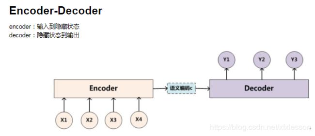
Sequence to Sequence模型
训练：训练时decoder每个单元输出得到的单词并不！作为下一个单元的输入单词。

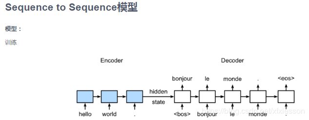
预测：Encoder的隐层状态准确性奠定了翻译的准确性

Seq2Seq具体结构：其中Embbedding层把每个单词序列映射成一个n维向量。

class Seq2SeqEncoder(d2l.Encoder):
    def __init__(self, vocab_size, embed_size, num_hiddens, num_layers,
                 dropout=0, **kwargs):
        super(Seq2SeqEncoder, self).__init__(**kwargs)
        self.num_hiddens = num_hiddens
        self.num_layers = num_layers
        # self.embedding.weight是vocab_size*embed_size的字典，
        # 每行对应应索引为0~vocab_size-1的词向量。
        # 思考：词向量的映射是固定的还是随着训练更新？——requires_grad=True
        self.embedding = nn.Embedding(vocab_size, embed_size)
        self.rnn = nn.LSTM(
            embed_size, # input_size
            num_hiddens,
            num_layers,
            dropout=dropout)

    def begin_state(self, batch_size, device):
        return [torch.zeros(size=(self.num_layers, batch_size, self.num_hiddens),  device=device),
                torch.zeros(size=(self.num_layers, batch_size, self.num_hiddens),  device=device)]

    def forward(self, X, *args):
        X = self.embedding(X)  # X shape: (batch_size, seq_len, embed_size)
        X = X.transpose(0, 1)  # RNN needs first axes to be time
        # X shape: (seq_len, batch_size, embed_size)
        # state = self.begin_state(X.shape[1], device=X.device)
        out, state = self.rnn(X)
        # The shape of out is (seq_len, batch_size, num_hiddens).
        # state contains the hidden state and the memory cell
        # of the last time step, the shape is (num_layers, batch_size, num_hiddens)
        return out, state
# vocab_size是词典长度
encoder = Seq2SeqEncoder(vocab_size=10, embed_size=8,num_hiddens=16, num_layers=2)
# (batch_size, seq_len）
X = torch.zeros((4, 7),dtype=torch.long)
# 为什么可以这样？而不是encoder.forward(X)
output, state = encoder(X)
output.shape, len(state), state[0].shape, state[1].shape
#(torch.Size([7, 4, 16]), 2, torch.Size([2, 4, 16]), torch.Size([2, 4, 16]))

encoder = Seq2SeqEncoder(vocab_size=10, embed_size=8,num_hiddens=16, num_layers=2)
X = torch.zeros((4, 7),dtype=torch.long)
output, state = encoder(X)
output.shape, len(state), state[0].shape, state[1].shape

2、注意力机制与Seq2seq模型

1、注意力机制

①引入背景
在“编码器—解码器（seq2seq），解码器在各个时间步依赖相同的背景变量（context vector）来获取输入序列信息。
RNN机制实际中存在长程梯度消失的问题，对于较长的句子，我们很难寄希望于将输入的序列转化为定长的向量而保存所有的有效信息，所以随着所需翻译句子的长度的增加，这种结构的效果会显著下降。

与此同时，解码的目标词语可能只与原输入的部分词语有关，而并不是与所有的输入有关。例如，当把“Hello world”翻译成“Bonjour le monde”时，“Hello”映射成“Bonjour”，“world”映射成“monde”。在seq2seq模型中，解码器只能隐式地从编码器的最终状态中选择相应的信息。然而，注意力机制可以将这种选择过程显式地建模。

②注意力机制框架

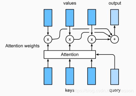
• Attention 是一种通用的带权池化方法。
• 输入由两部分构成：询问（query）和键值对（key-value pairs）。
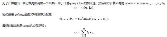
• Query ∈ℝ , ∈ℝ，∈ℝ， 最终输出∈ℝ。
• 对于一个query来说，attention layer 会与每一个key计算注意力分数并进-行权重的归一化，输出的向量o则是value的加权求和，而每个key计算的权重与value一一对应。
• 不同的attetion layer的区别在于score函数的选择。
  
  ③Softmax屏蔽：只对padding前的有效字符计算softmax。

masked_softmax(X, valid_length)

超出2维矩阵的乘法——批量乘法。X 和 Y 是维度分别为(b,n,m) 和(b,m,k)的张量，进行 b 次二维矩阵乘法后得到 Z, 维度为 (b,n,k)。

2、点积注意力
假设query和keys有相同的维度, 即 ∀i,,∈ℝ. 通过计算query和key转置的乘积来计算attention score,通常还会除去 d 减少计算出来的score对维度的依赖性。

假设∈ℝ×有m个query，∈ℝ×有n个keys. 我们可以通过矩阵运算的方式计算所有mn个score：

# Save to the d2l package.
class DotProductAttention(nn.Module): 
    def __init__(self, dropout, **kwargs):
        super(DotProductAttention, self).__init__(**kwargs)
        self.dropout = nn.Dropout(dropout)

    # query: (batch_size, #queries, d)
    # key: (batch_size, #kv_pairs, d)
    # value: (batch_size, #kv_pairs, dim_v)
    # valid_length: either (batch_size, ) or (batch_size, xx)
    def forward(self, query, key, value, valid_length=None):
        d = query.shape[-1]
        # set transpose_b=True to swap the last two dimensions of key
        
        scores = torch.bmm(query, key.transpose(1,2)) / math.sqrt(d)
        attention_weights = self.dropout(masked_softmax(scores, valid_length))
        print("attention_weight\n",attention_weights)
        return torch.bmm(attention_weights, value)
atten = DotProductAttention(dropout=0)

keys = torch.ones((2,10,2),dtype=torch.float)
values = torch.arange((40), dtype=torch.float).view(1,10,4).repeat(2,1,1)
atten(torch.ones((2,1,2),dtype=torch.float), keys, values, torch.FloatTensor([2, 6]))
[out]:
attention_weight
 tensor([[[0.5000, 0.5000, 0.0000, 0.0000, 0.0000, 0.0000, 0.0000, 0.0000,
          0.0000, 0.0000]],

        [[0.1667, 0.1667, 0.1667, 0.1667, 0.1667, 0.1667, 0.0000, 0.0000,
          0.0000, 0.0000]]])
tensor([[[ 2.0000,  3.0000,  4.0000,  5.0000]],

        [[10.0000, 11.0000, 12.0000, 13.0000]]])

3、多层感知机注意力
首先将 query and keys 投影到 ℝℎ ，做如下映射 ∈ℝℎ× , ∈ℝℎ× , and ∈ℝh . 将score函数定义

然后将key 和 value 在特征的维度上合并（concatenate），然后送至 a single hidden layer perceptron 这层中 hidden layer 为 ℎ and 输出size为 1 .隐层激活函数为tanh，无偏置.

# Save to the d2l package.
class MLPAttention(nn.Module):  
    def __init__(self, units,ipt_dim,dropout, **kwargs):
        super(MLPAttention, self).__init__(**kwargs)
        # Use flatten=True to keep query's and key's 3-D shapes.
        self.W_k = nn.Linear(ipt_dim, units, bias=False)
        self.W_q = nn.Linear(ipt_dim, units, bias=False)
        self.v = nn.Linear(units, 1, bias=False)
        self.dropout = nn.Dropout(dropout)

    def forward(self, query, key, value, valid_length):
        # size torch.Size([2, 1, 8]) torch.Size([2, 10, 8])
        query, key = self.W_k(query), self.W_q(key)
        # expand query to (batch_size, #querys, 1, units), and key to
        # (batch_size, 1, #kv_pairs, units). Then plus them with broadcast.
        # (2,1,10,8)
        features = query.unsqueeze(2) + key.unsqueeze(1)   
        #scores: torch.Size([2, 1, 10])     
        scores = self.v(features).squeeze(-1) 
        attention_weights = self.dropout(masked_softmax(scores, valid_length))
        return torch.bmm(attention_weights, value)
atten = MLPAttention(ipt_dim=2,units = 8, dropout=0)
keys = torch.ones((2,10,2),dtype=torch.float)
values = torch.arange((40), dtype=torch.float).view(1,10,4).repeat(2,1,1)

atten(torch.ones((2,1,2), dtype = torch.float), keys, values, torch.FloatTensor([2, 6]))
[out]:
tensor([[[ 2.0000,  3.0000,  4.0000,  5.0000]],

        [[10.0000, 11.0000, 12.0000, 13.0000]]], grad_fn=<BmmBackward>)

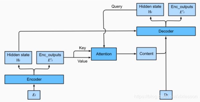
4、引入注意力机制的Seq2seq模型
本节中将注意机制添加到sequence to sequence 模型中，以显式地使用权重聚合states。

下图展示encoding 和decoding的模型结构，在时间步为t的时候。此刻attention layer保存着encodering看到的所有信息——即encoding的每一步输出。在decoding阶段，解码器的t时刻的隐藏状态被当作query，encoder的每个时间步的hidden states作为key和value进行attention聚合. Attetion model的输出当作成上下文信息context vector，并与解码器输入Dt拼接起来一起送到解码器：

class Seq2SeqAttentionDecoder(d2l.Decoder):
    def __init__(self, vocab_size, embed_size, num_hiddens, num_layers,
                 dropout=0, **kwargs):
        super(Seq2SeqAttentionDecoder, self).__init__(**kwargs)
        self.attention_cell = MLPAttention(num_hiddens,num_hiddens, dropout)
        self.embedding = nn.Embedding(vocab_size, embed_size)
        self.rnn = nn.LSTM(embed_size+ num_hiddens,num_hiddens, num_layers, dropout=dropout)
        self.dense = nn.Linear(num_hiddens,vocab_size)

    def init_state(self, enc_outputs, enc_valid_len, *args):
        outputs, hidden_state = enc_outputs
#         print("first:",outputs.size(),hidden_state[0].size(),hidden_state[1].size())
        # Transpose outputs to (batch_size, seq_len, hidden_size)
        return (outputs.permute(1,0,-1), hidden_state, enc_valid_len)
        #outputs.swapaxes(0, 1)
        
    def forward(self, X, state):
        enc_outputs, hidden_state, enc_valid_len = state
        #("X.size",X.size())
        X = self.embedding(X).transpose(0,1)
#         print("Xembeding.size2",X.size())
        outputs = []
        for l, x in enumerate(X):
#             print(f"\n{l}-th token")
#             print("x.first.size()",x.size())
            # query shape: (batch_size, 1, hidden_size)
            # select hidden state of the last rnn layer as query
            query = hidden_state[0][-1].unsqueeze(1) 
            # np.expand_dims(hidden_state[0][-1], axis=1)
            # context has same shape as query
            context = self.attention_cell(query, enc_outputs, enc_outputs, enc_valid_len)
            # Concatenate on the feature dimension
#             print("context.size:",context.size())
            x = torch.cat((context, x.unsqueeze(1)), dim=-1)
            # Reshape x to (1, batch_size, embed_size+hidden_size)
#             print("rnn",x.size(), len(hidden_state))
            out, hidden_state = self.rnn(x.transpose(0,1), hidden_state)
            outputs.append(out)
        outputs = self.dense(torch.cat(outputs, dim=0))
        return outputs.transpose(0, 1), [enc_outputs, hidden_state,
                                        enc_valid_len]

3、Transformer

1、Transformer的引入

• CNNs 易于并行化，却不适合捕捉变长序列内的依赖关系。
• RNNs 适合捕捉长距离变长序列的依赖，但是却难以实现并行化处理序列。

为了整合CNN和RNN的优势，[Vaswani et al., 2017] 创新性地使用注意力机制设计了Transformer模型。该模型利用attention机制实现了并行化捕捉序列依赖，并且同时处理序列的每个位置的tokens，上述优势使得Transformer模型在性能优异的同时大大减少了训练时间。

Transformer模型与seq2seq模型的区别主要在于以下三点：

• Transformer blocks：将seq2seq模型重的循环网络替换为了Transformer Blocks，该模块包含一个多头注意力层（Multi-head Attention Layers）以及两个position-wise feed-forward networks（FFN）。对于解码器来说，另一个多头注意力层被用于接受编码器的隐藏状态。
• Add and norm：多头注意力层和前馈网络的输出被送到两个“add and norm”层进行处理，该层包含残差结构以及层归一化。
• Position encoding：由于自注意力层并没有区分元素的顺序，所以一个位置编码层被用于向序列元素里添加位置信息。

2、多头注意力层

• 自注意力（self-attention）模型是一个正规的注意力模型，序列的每一个元素对应的key，value，query是完全一致的。
• 下图中，自注意力层输出了一个与输入长度相同的表征序列，与循环神经网络相比，自注意力对每个元素输出的计算是并行的，所以我们可以高效的实现这个模块。
  
• 多头注意力层包含h个并行的自注意力层，每一个这种层被成为一个head。
• 对每个头来说，在进行注意力计算之前，我们会将query、key和value用三个现行层进行映射，这h个注意力头的输出将会被拼接之后输入最后一个线性层进行整合。
• 多头注意力层保持输入与输出张量的维度不变，只会对最后一维的大小进行改变。
  

class MultiHeadAttention(nn.Module):
    def __init__(self, input_size, hidden_size, num_heads, dropout, **kwargs):
        super(MultiHeadAttention, self).__init__(**kwargs)
        self.num_heads = num_heads
        self.attention = DotProductAttention(dropout)
        self.W_q = nn.Linear(input_size, hidden_size, bias=False)
        self.W_k = nn.Linear(input_size, hidden_size, bias=False)
        self.W_v = nn.Linear(input_size, hidden_size, bias=False)
        self.W_o = nn.Linear(hidden_size, hidden_size, bias=False)
    
    def forward(self, query, key, value, valid_length):
        # query, key, and value shape: (batch_size, seq_len, dim),
        # where seq_len is the length of input sequence
        # valid_length shape is either (batch_size, )
        # or (batch_size, seq_len).

        # Project and transpose query, key, and value from
        # (batch_size, seq_len, hidden_size * num_heads) to
        # (batch_size * num_heads, seq_len, hidden_size).
        
        query = transpose_qkv(self.W_q(query), self.num_heads)
        key = transpose_qkv(self.W_k(key), self.num_heads)
        value = transpose_qkv(self.W_v(value), self.num_heads)
        
        if valid_length is not None:
            # Copy valid_length by num_heads times
            device = valid_length.device
            valid_length = valid_length.cpu().numpy() if valid_length.is_cuda
                                                    else valid_length.numpy()
            if valid_length.ndim == 1:
                valid_length = torch.FloatTensor(np.tile(valid_length, self.num_heads))
            else:
                valid_length = torch.FloatTensor(np.tile(valid_length, (self.num_heads,1)))

            valid_length = valid_length.to(device)
            
        output = self.attention(query, key, value, valid_length)
        output_concat = transpose_output(output, self.num_heads)
        return self.W_o(output_concat)
# input_size, hidden_size, num_heads, dropout
cell = MultiHeadAttention(5, 9, 3, 0.5)
# (batch_size, seq_len, input_size)
X = torch.ones((2, 4, 5))
valid_length = torch.FloatTensor([2, 3])
# (batch_size, seq_len, hidden_size)
cell(X, X, X, valid_length).shape
[out]:
torch.Size([2, 4, 9])

3、基于位置的前馈网络（PositionWiseFFN）

• Position-wise FFN由两个全连接层组成，他们作用在最后一维上。因为序列的每个位置的状态都会被单独地更新，所以我们称他为position-wise，这等效于一个1x1的卷积。
• 对于两个完全相同的输入，FFN层的输出也将相等。

# Save to the d2l package.
class PositionWiseFFN(nn.Module):
    def __init__(self, input_size, ffn_hidden_size, hidden_size_out, **kwargs):
        super(PositionWiseFFN, self).__init__(**kwargs)
        self.ffn_1 = nn.Linear(input_size, ffn_hidden_size)
        self.ffn_2 = nn.Linear(ffn_hidden_size, hidden_size_out)
                
    def forward(self, X):
        return self.ffn_2(F.relu(self.ffn_1(X)))
ffn = PositionWiseFFN(4, 4, 8)
out = ffn(torch.ones((2,3,4)))

print(out, out.shape)  # torch.Size([2, 3, 8]

4、Add and Norm：

• 相加归一化层，它可以平滑地整合输入和其他层的输出，因此我们在每个多头注意力层和FFN层后面都添加一个含残差连接的Layer Norm层。
• Batch Norm是对于batch size这个维度进行计算均值和方差的，而Layer Norm则是对最后一维进行计算（nn.LayerNorm）。
• 层归一化可以防止层内的数值变化过大，从而有利于加快训练速度并且提高泛化性能。

# Save to the d2l package.
class AddNorm(nn.Module):
    def __init__(self, hidden_size, dropout, **kwargs):
        super(AddNorm, self).__init__(**kwargs)
        self.dropout = nn.Dropout(dropout)
        self.norm = nn.LayerNorm(hidden_size)
    # 由于残差连接，X和Y需要有相同的维度。
    def forward(self, X, Y):
        return self.norm(self.dropout(Y) + X)
add_norm = AddNorm(4, 0.5)
add_norm(torch.ones((2,3,4)), torch.ones((2,3,4))).shape
# torch.Size([2, 3, 4])

5、位置编码

• 与循环神经网络不同，无论是多头注意力网络还是前馈神经网络都是独立地对每个位置的元素进行更新，这种特性帮助我们实现了高效的并行，却丢失了重要的序列顺序的信息。
• 为了更好的捕捉序列信息，Transformer模型引入了位置编码去保持输入序列元素的位置。
• 假设输入序列的嵌入表示 X∈Rl×d, 序列长度为l嵌入向量维度为d，则其位置编码为P∈Rl×d ，输出的向量就是二者相加 X+P。

6、编码器

• Encoder Block：多头注意力层+Add and Norm+Position-wise FFN+Add and Norm。
• 整个Transformer 编码器模型n个Encoder Block堆叠而成。
• 因为残差连接的缘故，中间状态的维度始终与嵌入向量的维度d一致；同时把嵌入向量乘以d**0.5以防止其值过小。

class TransformerEncoder(d2l.Encoder):
    def __init__(self, vocab_size, embedding_size, ffn_hidden_size,
                 num_heads, num_layers, dropout, **kwargs):
        super(TransformerEncoder, self).__init__(**kwargs)
        self.embedding_size = embedding_size
        self.embed = nn.Embedding(vocab_size, embedding_size)
        self.pos_encoding = PositionalEncoding(embedding_size, dropout)
        self.blks = nn.ModuleList()
        for i in range(num_layers):
            self.blks.append(
                EncoderBlock(embedding_size, ffn_hidden_size,
                             num_heads, dropout))

    def forward(self, X, valid_length, *args):
        # torch.Size([2, 100, 24])
        X = self.pos_encoding(self.embed(X) * math.sqrt(self.embedding_size))
        for blk in self.blks:
            X = blk(X, valid_length)
        return X
# test encoder
encoder = TransformerEncoder(200, 24, 48, 8, 2, 0.5)
encoder(torch.ones((2, 100)).long(), valid_length).shape
# torch.Size([2, 100, 24])

7、解码器

Transformer 模型的解码器与编码器结构类似，然而，除了之前介绍的几个模块之外，编码器部分有另一个子模块。该模块也是多头注意力层，接受编码器的输出作为key和value，decoder的状态作为query。与编码器部分相类似，解码器同样是使用了add and norm机制，用残差和层归一化将各个子层的输出相连。

仔细来讲，在第t个时间步，当前输入xt是query，那么self attention接受了第t步以及前t-1步的所有输入x1,…,xt−1。在训练时，由于第t位置的输入可以观测到全部的序列，这与预测阶段的情形项矛盾，所以我们要通过将第t个时间步所对应的可观测长度设置为t，以消除不需要看到的未来的信息。

class DecoderBlock(nn.Module):
    def __init__(self, embedding_size, ffn_hidden_size, num_heads,dropout,i,**kwargs):
        super(DecoderBlock, self).__init__(**kwargs)
        self.i = i
        self.attention_1 = MultiHeadAttention(embedding_size, embedding_size, num_heads, dropout)
        self.addnorm_1 = AddNorm(embedding_size, dropout)
        self.attention_2 = MultiHeadAttention(embedding_size, embedding_size, num_heads, dropout)
        self.addnorm_2 = AddNorm(embedding_size, dropout)
        self.ffn = PositionWiseFFN(embedding_size, ffn_hidden_size, embedding_size)
        self.addnorm_3 = AddNorm(embedding_size, dropout)
    
    def forward(self, X, state):
        enc_outputs, enc_valid_length = state[0], state[1]
        
        # state[2][self.i] stores all the previous t-1 query state of layer-i
        # len(state[2]) = num_layers
        
        # If training:
        #     state[2] is useless.
        # If predicting:
        #     In the t-th timestep:
        #         state[2][self.i].shape = (batch_size, t-1, hidden_size)
        # Demo:
        # love dogs ! [EOS]
        #  |    |   |   |
        #   Transformer 
        #    Decoder
        #  |   |   |   |
        #  I love dogs !
        
        if state[2][self.i] is None:
            key_values = X
        else:
            # shape of key_values = (batch_size, t, hidden_size)
            key_values = torch.cat((state[2][self.i], X), dim=1) 
        state[2][self.i] = key_values
        
        if self.training:
            batch_size, seq_len, _ = X.shape
            # Shape: (batch_size, seq_len), the values in the j-th column are j+1
            valid_length = torch.FloatTensor(np.tile(np.arange(1, seq_len+1), (batch_size, 1))) 
            valid_length = valid_length.to(X.device)
        else:
            valid_length = None

        X2 = self.attention_1(X, key_values, key_values, valid_length)
        Y = self.addnorm_1(X, X2)
        Y2 = self.attention_2(Y, enc_outputs, enc_outputs, enc_valid_length)
        Z = self.addnorm_2(Y, Y2)
        return self.addnorm_3(Z, self.ffn(Z)), state