数据分析入门之KNN-预测年收入
文章目录
- 1、导入数据
- 2、数据预处理
- 2.1、选择数据
- 2.2、数据转化
- 2.2.1、转化字典
- 2.2.2、数据映射
- 3、训练数据
- 3.1、切分训练集和测试集
- 3.2、训练并预测数据
- 4、归一化处理
- 4.1、最大值最小值归一化
- 4.2、方差标准化
- 5、保存模型与调用
- 5.1、保存模型
- 5.2、加载模型
- 5.3、使用预测
操作平台: win10, python37, jupyter
数据下载: https://www.lanzous.com/iac0omd
1、导入数据
import numpy as np
import pandas as pd
from sklearn.neighbors import KNeighborsClassifier
salary = pd.read_csv('../data/adults.txt')
salary.shape # 结果为(32561, 15)
salary.head() #展示前5行
| age | workclass | final_weight | education | education_num | marital_status | occupation | relationship | race | sex | capital_gain | capital_loss | hours_per_week | native_country | salary | |
|---|---|---|---|---|---|---|---|---|---|---|---|---|---|---|---|
| 0 | 39 | State-gov | 77516 | Bachelors | 13 | Never-married | Adm-clerical | Not-in-family | White | Male | 2174 | 0 | 40 | United-States | <=50K |
| 1 | 50 | Self-emp-not-inc | 83311 | Bachelors | 13 | Married-civ-spouse | Exec-managerial | Husband | White | Male | 0 | 0 | 13 | United-States | <=50K |
| 2 | 38 | Private | 215646 | HS-grad | 9 | Divorced | Handlers-cleaners | Not-in-family | White | Male | 0 | 0 | 40 | United-States | <=50K |
| 3 | 53 | Private | 234721 | 11th | 7 | Married-civ-spouse | Handlers-cleaners | Husband | Black | Male | 0 | 0 | 40 | United-States | <=50K |
| 4 | 28 | Private | 338409 | Bachelors | 13 | Married-civ-spouse | Prof-specialty | Wife | Black | Female | 0 | 0 | 40 | Cuba | <=50K |
2、数据预处理
2.1、选择数据
- 选择影响薪水相关性较大的数据来作为X,进行预测薪水 y :
y = salary['salary']
X = salary.iloc[:,[0,1,3,5,6,8,9,-2,-3]]
X.head()
| age | workclass | education | marital_status | occupation | race | sex | native_country | hours_per_week | |
|---|---|---|---|---|---|---|---|---|---|
| 0 | 39 | State-gov | Bachelors | Never-married | Adm-clerical | White | Male | United-States | 40 |
| 1 | 50 | Self-emp-not-inc | Bachelors | Married-civ-spouse | Exec-managerial | White | Male | United-States | 13 |
| 2 | 38 | Private | HS-grad | Divorced | Handlers-cleaners | White | Male | United-States | 40 |
| 3 | 53 | Private | 11th | Married-civ-spouse | Handlers-cleaners | Black | Male | United-States | 40 |
| 4 | 28 | Private | Bachelors | Married-civ-spouse | Prof-specialty | Black | Female | Cuba | 40 |
查看数据类型
X.info()
<class 'pandas.core.frame.DataFrame'>
RangeIndex: 32561 entries, 0 to 32560
Data columns (total 9 columns):
age               32561 non-null int64
workclass         32561 non-null int64
education         32561 non-null int64
marital_status    32561 non-null int64
occupation        32561 non-null int64
race              32561 non-null int64
sex               32561 non-null int64
native_country    32561 non-null int64
hours_per_week    32561 non-null int64
dtypes: int64(9)
memory usage: 2.2 MB
knn = KNeighborsClassifier()

knn.fit(X,y)
结果分析: 上面的数据大多都是字符型,不能直接进行数据运算,需要进行数据的转换!
2.2、数据转化
- 把它出现的字符数据分别用对用的值来替代
2.2.1、转化字典
workclass = X['workclass'].unique()
m = {}
for i,work in enumerate(workclass):
    m[work] = i
m
{'State-gov': 0,
 'Self-emp-not-inc': 1,
 'Private': 2,
 'Federal-gov': 3,
 'Local-gov': 4,
 '?': 5,
 'Self-emp-inc': 6,
 'Without-pay': 7,
 'Never-worked': 8}
结果分析: 用0代表职业State-gov,1代表Self-emp-not-inc,2代表Private等等。
2.2.2、数据映射
X['workclass'] = X['workclass'].map(m)
X.head()
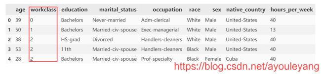
结果分析: 现在工作机构已经被映射为对应的数字了,接下了再把其他几个也映射为对应的数字。
列如:
u = X['occupation'].unique()
np.argwhere(u == 'Sales')[0,0]
5
实例:
for col in X.columns[2:-1]:

    u = X[col].unique()

    def convert(x):
        return np.argwhere(u == x)[0,0]

    X[col] = X[col].map(convert)
X.head()
| age | workclass | education | marital_status | occupation | race | sex | native_country | hours_per_week | |
|---|---|---|---|---|---|---|---|---|---|
| 0 | 39 | 0 | 0 | 0 | 0 | 0 | 0 | 0 | 40 |
| 1 | 50 | 1 | 0 | 1 | 1 | 0 | 0 | 0 | 13 |
| 2 | 38 | 2 | 1 | 2 | 2 | 0 | 0 | 0 | 40 |
| 3 | 53 | 2 | 2 | 1 | 2 | 1 | 0 | 0 | 40 |
| 4 | 28 | 2 | 0 | 1 | 3 | 1 | 1 | 1 | 40 |
3、训练数据
3.1、切分训练集和测试集
from sklearn.model_selection import train_test_split
# X -----> y一一对应
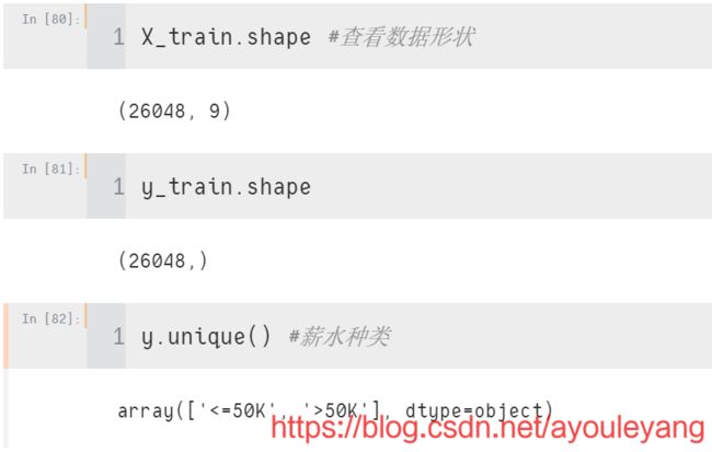
X_train,X_test,y_train,y_test = train_test_split(X,y,test_size = 0.2)
3.2、训练并预测数据
knn = KNeighborsClassifier(n_neighbors=5) #邻近值为5,可以变化邻近值,加上weights='distance'等

knn.fit(X_train,y_train)#训练模型

y_ = knn.predict(X_test)#预测数据

result = y_ == y_test #对比测试集和预测集,返回True和False

result.mean()#求平均值,代表准确率
0.7690772301550745
4、归一化处理
4.1、最大值最小值归一化
v_min = X.min()
v_max = X.max()
X2 = (X - v_min)/(v_max - v_min)
X2.head()
| age | workclass | education | marital_status | occupation | race | sex | native_country | hours_per_week | |
|---|---|---|---|---|---|---|---|---|---|
| 0 | 0.301370 | 0.000 | 0.000000 | 0.000000 | 0.000000 | 0.00 | 0.0 | 0.00000 | 0.397959 |
| 1 | 0.452055 | 0.125 | 0.000000 | 0.166667 | 0.071429 | 0.00 | 0.0 | 0.00000 | 0.122449 |
| 2 | 0.287671 | 0.250 | 0.066667 | 0.333333 | 0.142857 | 0.00 | 0.0 | 0.00000 | 0.397959 |
| 3 | 0.493151 | 0.250 | 0.133333 | 0.166667 | 0.142857 | 0.25 | 0.0 | 0.00000 | 0.397959 |
| 4 | 0.150685 | 0.250 | 0.000000 | 0.166667 | 0.214286 | 0.25 | 1.0 | 0.02439 | 0.397959 |
数据预测:
# 归一化,消除属性差异
X_train,X_test,y_train,y_test = train_test_split(X2,y,test_size = 0.2)
knn = KNeighborsClassifier(n_neighbors=15,weights='distance')

knn.fit(X_train,y_train)

y_ = knn.predict(X_test)

result = y_ == y_test

result.mean()
0.8174420389989252
自带方法:
from sklearn.preprocessing import MinMaxScaler

m = MinMaxScaler()
X4 = m.fit_transform(X)
X4[:5]
array([[0.30136986, 0.        , 0.        , 0.        , 0.        ,
        0.        , 0.        , 0.        , 0.39795918],
       [0.45205479, 0.125     , 0.        , 0.16666667, 0.07142857,
        0.        , 0.        , 0.        , 0.12244898],
       [0.28767123, 0.25      , 0.06666667, 0.33333333, 0.14285714,
        0.        , 0.        , 0.        , 0.39795918],
       [0.49315068, 0.25      , 0.13333333, 0.16666667, 0.14285714,
        0.25      , 0.        , 0.        , 0.39795918],
       [0.15068493, 0.25      , 0.        , 0.16666667, 0.21428571,
        0.25      , 1.        , 0.02439024, 0.39795918]])
4.2、方差标准化
# Z-score
v_mean = X.mean()

v_std = X.std()

X3 = (X - v_mean)/v_std
X3.head()
| age | workclass | education | marital_status | occupation | race | sex | native_country | hours_per_week | |
|---|---|---|---|---|---|---|---|---|---|
| 0 | 0.030670 | -1.884571 | -0.991569 | -0.866068 | -1.378100 | -0.353403 | -0.703061 | -0.255743 | -0.035429 |
| 1 | 0.837096 | -1.068730 | -0.991569 | -0.066951 | -1.082777 | -0.353403 | -0.703061 | -0.255743 | -2.222119 |
| 2 | -0.042641 | -0.252888 | -0.702015 | 0.732166 | -0.787453 | -0.353403 | -0.703061 | -0.255743 | -0.035429 |
| 3 | 1.057031 | -0.252888 | -0.412460 | -0.066951 | -0.787453 | 1.240608 | -0.703061 | -0.255743 | -0.035429 |
| 4 | -0.775756 | -0.252888 | -0.991569 | -0.066951 | -0.492130 | 1.240608 | 1.422309 | -0.057541 | -0.035429 |
数据预测:
X_train,X_test,y_train,y_test = train_test_split(X3,y,test_size = 0.2)
knn = KNeighborsClassifier(n_neighbors=15,weights='distance')

knn.fit(X_train,y_train)

y_ = knn.predict(X_test)

result = y_ == y_test

result.mean()
0.8106863196683556
自带方法:
from sklearn.preprocessing import StandardScaler

s = StandardScaler()
X5 = s.fit_transform(X)
X5[:5]
array([[ 0.03067056, -1.88460023, -0.99158435, -0.8660817 , -1.37812112,
        -0.35340882, -0.70307135, -0.25574647, -0.03542945],
       [ 0.83710898, -1.0687461 , -0.99158435, -0.06695205, -1.08279326,
        -0.35340882, -0.70307135, -0.25574647, -2.22215312],
       [-0.04264203, -0.25289198, -0.70202542,  0.7321776 , -0.78746539,
        -0.35340882, -0.70307135, -0.25574647, -0.03542945],
       [ 1.05704673, -0.25289198, -0.4124665 , -0.06695205, -0.78746539,
         1.240627  , -0.70307135, -0.25574647, -0.03542945],
       [-0.77576787, -0.25289198, -0.99158435, -0.06695205, -0.49213753,
         1.240627  ,  1.42233076, -0.05754204, -0.03542945]])
5、保存模型与调用
5.1、保存模型
from sklearn.externals import joblib
joblib.dump(knn,'./model')
['./model']
5.2、加载模型
model = joblib.load('./model')
model
5.3、使用预测
model.score(X_test,y_test)
0.8174420389989252
保存为其他格式:
