Representation Flow for Action Recognition —— 翻译

“
该论文发表在CVPR 2019上，本文主要对该论文进行段落逐字翻译。
论文下载： 论文下载地址.
CV小白初入CV，还请多指教。
”

Abstract 摘要

• In this paper, we propose a convolutional layer inspired by optical flow algorithms to learn motion representations. Our representation flow layer is a fully-differentiable layer designed to capture the ‘flow’ of any representation channel within a convolutional neural network for action recognition. Its parameters for iterative flow optimization are learned in an end-to-end fashion together with the other CNN model parameters, maximizing the action recognition performance. Furthermore, we newly introduce the concept of learning ‘flow of flow’ representations by stacking multiple representation flow layers. We conducted extensive experimental evaluations, confirming its advantages over previous recognition models using traditional optical flows in both computational speed and performance. The code is publicly available.
• 在本文中，我们提出了一个受光流法启发的学习运动特征的卷积层。我们的表示流层是一个完全可微的层，被设计用来捕捉在卷积神经网络中任何通道的光流进行行为识别。它的迭代流优化参数和其他CNN模型的参数一起以端到端的方式学习，以此来最大化行为识别性能。而且，我们最新提出了 ‘flow to flow’ 的概念，是通过叠加多个表示流层表示的。我们进行了大量实验评估证明该方法的计算速度和性能优于先前使用传统光流方法的识别模型。该方法的代码是公开可用的。

1 Introduction 简介

• Activity recognition is an important problem in computer vision with many societal applications including surveillance, robot perception, smart environment/city, and more. Use of video convolutional neural networks (CNNs) have become the standard method for this task, as they can learn more optimal representations for the problem. Two-stream networks[20], taking both RGB frames and optical flow as input, provide state-of-the-art results and have been extremely popular.3-D spatio-temporal CNN models, e.g., I3D [3] , with XYT convolutions also found that such two-stream design (RGB + optical flow) increases their accuracy. Abstracting both appearance information and explicit motion flow benefits the recognition.

• 行为识别在计算机视觉中是一个非常重要的问题，在监视、机器感知、智慧环境/城市等诸多社会应用中都有所应用。使用视频卷积神经网络（CNNs）已经成为完成该任务的标准方法，因为该方法可以学习到问题更优的特征。双流网络以RGB帧和光流作为输入，该方法得到了非常先进的结果而且非常流行。3D时空卷积模型，比如使用XYT三个维度的I3D也发现了双流设计（RGB+光流）提高了精度。将外观信息和运动流信息抽象出来有利于识别。

• However, optical flow is expensive to compute. It often requires hundreds of optimization iterations every frame, and causes learning of two separate CNN streams (i.e., RGB-stream and flow-stream). This requires significant computation cost and a great increase in the number of model parameters to learn. Further, this means that the model needs to compute optical flow every frame even during inference and run two parallel CNNs, limiting its real-time applications.

• 然而，光流的计算开销大。它通常要求对每一帧进行几百次的最优迭代，而且需要学习两个独立的卷积流（即，RGB流和光流）。这需要大量的计算成本和足够的模型参数训练。此外，这代表该模型需要在判断的时候计算每一帧的光流，而且同时运行两个CNNs，这些限制了它的实时应用。

• There were previous works to learn representations capturing motion information without using optical flow as input, such as motion feature networks [15] and ActionFlowNet[16]. However, although they were more advantageous in terms of the number of model parameters and computation speed, they suffered from inferior performance compared to two-stream models on public datasets such as Kinetics [13] and HMDB [14]. We hypothesize that the iterative optimization performed by optical flow methods produces an important feature that other methods fail to capture.

• 先前有些工作，比如运动特征网络和ActionFlowNet捕获运动信息没有使用光流作为输入。然而，尽管它们在模型参数数量和计算速度上具有优势，但是与双流网络相比，在公共数据集Kinetics和HMDB上其性能较差。我们设想光流方法的迭代优化产生了一种其他方法不能捕获的重要特征。

• In this paper, we propose a CNN layer inspired by optical flow algorithms to learn motion representations for action recognition without having to compute optical flow. Our representation flow layer is a fully-differentiable layer designed to capture ‘flow’ of any representation channels within the
  model. Its parameters for iterative flow optimization are learned together with other model parameters, maximizing the action recognition performance. This is also done without having/training multiple network streams, reducing the number of parameters in the model. Further, we newly introduce the concept of learning ‘flow of flow’ representations by stacking multiple representation flow layers. We conduct extensive action classification experimental evaluation of where to compute optical flow and various hyperparameters, learning parameters, and fusion techniques.

• 在这篇文章中，我们受通过光流法学习运动特征启发，提出了不需要计算光流来进行行为识别的CNN层。我们的表示流层是一个完全可微的层，被设计用来捕捉在卷积神经网络中任何通道的光流进行行为识别。它的迭代流优化参数和其他CNN模型的参数一起以端到端的方式学习，以此来最大化行为识别性能。同样这也不需要有/训练多个网络流，因此减少了模型的参数。而且，我们最新提出了 ‘flow to flow’ 的概念，是通过叠加多个表示流层表示的。我们进行大量行为识别实验，评估哪里适合计算光流和各种超参数、学习参数和融合技术。

• Our contribution is the introduction of a new differentiable CNN layer that unrolls the iterations of the TV-L1 optical flow method. This allows for learning of the optical flow parameters, application to any CNN feature maps (i.e., intermediate representations), and lower computational cost while maintaining performance.

• 我们的贡献是引入了一个新的可微CNN层，这展开了TV-L1光流方法的迭代。这允许学习光流参数运用到任何CNN的特征地图（即，中间特征）以及在保持性能的同时产生更低的计算开销。

2 Related Works 相关工作

• Capturing motion and temporal information has been studied for activity recognition. Early, hand-crafted approaches such as dense trajectories [24] captured motion information by tracking points through time. Many algorithms have been developed to compute optical flow as a way to capture motion in video [8]. Other works have explored learning the ordering of frames to summarize a video in a single ‘dynamic image’ used for activity recognition [1].
• 捕获运动和时间特征早就在行为识别中被研究。早期，比如密集轨迹这一手工方法通过跟踪视频中的时间点来捕获运动信息。为了捕获视频中的运动信息，许多计算光流的方法被不断发展。也有其他工作探索了学习顺序帧去总结视频中的单一 ‘动态图像’ 来进行行为识别。
• Convolutional neural networks (CNNs) have been applied to activity recognition. Initial approaches explored methods to combine temporal information based on pooling or temporal convolution [12, 17]. Other works have explored using attention to capture sub-events of activities [18]. Two-stream
  networks have been very popular: they take input of a single RGB frame (captures appearance information) and a stack of optical flow frames (captures motion information). Often, the two network streams of the model are separately trained and the final predictions are averaged together [20]. There were other two-stream CNN works exploring different ways to ‘fuse’ or combine the motion CNN with the appearance CNN [7, 6]. There were also large 3D XYT CNNs learning spatio-temporal patterns [26, 3], enabled by large video datasets such as Kinetics [13]. However, these approaches
  still rely on optical flow input to maximize their accuracies.
• 卷积神经网络（CNNs）被应用在行为识别领域。最开始的结合时间特征的方法通过池化或者时间卷积来完成。其他工作也探索了使用注意力来获得行为的子事件。双流网络非常流行，是以单帧RGB帧（获得外观信息）和堆叠光流帧（获得运动型）作为输入。通常，两个网络需要单独训练，最后的预测结果是它们的平均值。也有其它双流网络探索使用不同的方法去融合或者结合运动CNN和外观CNN。也有大的3D XYT CNNs在大视频数据集（如，Kinetics）上来学习时空特征。然而，这些方法都依赖于将光流作为输入来获得最高的准确率。
• While optical flow is known to be an important feature, flows optimized for activity recognition are often different from the true optical flow [19], suggesting that end-to-end learning of motion representations is beneficial. Recently, there have been works on learning such motion representations using convolutional models. Fan et al. [5] implemented the TV-L1 method using deep learning libraries to increase its computational speed and allow for learning some parameters. The result was fed to a two-stream CNN for the recognition. Several works explored learning a CNN to predict optical flow, which also can be used for action recognition [4, 9, 11, 16, 21]. Lee et al. [15] shifted features from sequential frames to capture motion in a non-iterative fashion. Sun et al. [21] proposed an optical flow guided feature (OFF) by computing the gradients of representations and temporal differences, but it lacked the iterative optimization necessary for accurate flow computation. Further, it requires a three-stream model taking RGB, optical flow, and RGB differences to achieve state-of-the-art performance.
• 光流已被得知是一种非常重要的特征，但在行为识别中优化得到的光流往往与实际光流不同，这表明端到端的学习运动特征是有益的。最近，有使用卷积模型来学习这些运动特征。Fan等人通过使用深度学习库实施了TV-L1方法，以此提高了计算速度，也允许学习一些参数。结果被送入双流网络来进行行为识别。有一些工作通过学习CNN来预测光流，同样也被用于行为识别。Lee等人通过非迭代的方式获得运动特征。Sun等人提出通过计算特征梯度和时间差异的光流引导特征方法（OFF），但是该方法缺乏精确光流的必要迭代优化。而且它的最好性能需要RGB、光流以及RGB差异三种信息为输入的三流模型来获得。
• Unlike prior works, our proposed model with representation flow layers relies only on RGB input, learning far fewer parameters while correctly representing motion with the iterative optimization. It is significantly faster than the video CNNs requiring optical flow input, while still performing as good as or even better than the two-stream models. It clearly outperforms existing motion representation methods including TVNet [5] and OFF [21] in both speed and accuracy, which we experimentally confirm.
• 与先前的工作不同，我们提出的特征流层模型只依赖于RGB输入，在准确通过迭代优化获取运动特征时学习更少的参数。该方法比在视频CNNs中需要光流作为输入快很多，而且性能甚至好于双流模型。我们的实验证明，该方法在速度和精度上好于现有的运动特征方法，包括TVNet和OFF。

3 Approach 方法

• Our method is a fully-differentiable convolutional layer inspired by optical flow algorithms. Unlike traditional optical flow methods, all the parameters of our method can be learned end-to-end, maximizing action recognition performance. Furthermore, our layer is designed to compute the ‘flow’ of any representation channels, instead of limiting its input to be traditional RGB frames.
• 我们的方法是受光流法启发的一个完全可微的卷积层。与传统的光流方法不同，该方法的所有参数都可以进行端到端的学习来最大化识别的性能。而且，该方法不被限制以传统的RGB帧作为输入，可以计算任何一个特征通道的流。

3.1 Review of Optical Flow Methods 回顾光流方法

• Before describing our layer, we briefly review how optical flow is computed. Optical flow methods are based on the brightness consistency assumption. That is, given sequential images $I_1$, $I_2$, a point $x$, $y$ in $I_1$ is located at $x+∆x$, $y+∆y$ in $I_2$, or $I_1(x,y)=I_2(x+∆x,y+∆y)$. These methods assume small movements between frames, so this can be approximated with a Taylor series: $I_2=I_1+\frac{\delta I}{\delta x}∆x+\frac{\delta I}{\delta y}∆y$, where $u=[∆x,∆y]$. These equations are solved for $u$ to obtain the flow, but can only be approximated due to the two unknowns.
• 在讲述我们的层之前，我们先简单的回顾以下光流是如何计算的。光流法是基于光流一致性的假设。也就是说，给定序列图像 $I_1$, $I_2$，给定$I_1$中的两个点 $x$, $y$，其在$I_2$中的位置为$x+∆x$, $y+∆y$，即$I_1(x,y)=I_2(x+∆x,y+∆y)$。这些方法假设相邻帧之间是小位移的，所以可以使用泰勒级数近似表示：$I_2=I_1+\frac{\delta I}{\delta x}∆x+\frac{\delta I}{\delta y}∆y$，其中$u=[∆x,∆y]$。这些方程解$u$获得流信息，但因为两个未知数只能近似得到。
• The standard, variational methods for approximating optical flow (e.g., Brox [2] and TV-L1 [27] methods) take sequential images $I_1$, $I_2$ as input. Variational optical flow methods estimate the flow field, $u$, using an iterative optimization method. The tensor $u\in R^{2\times W\times H}$ is the $x$ and $y$ directional flow for every location in the image. Taking two sequential images as input, $I_1$, $I_2$, the methods first compute the gradient in both $x$ and $y$ directions: $\nabla I_2$. The initial flow is set to 0, $u=0$. Then $\rho$, which captures the motion residual between two frames, based on the current flow estimate $u$, can be computed. For efficiency, the constant part of $\rho$, ${\rho }_c$ is precomputed:
  $$\rho =I_2-{\nabla }_x{I}_2\cdot u_x-{\nabla }_y\cdot I_2\cdot u_y-I_1(1)$$
• 基于此的变异获得光流的方法（比如，Brox [2] 和 TV-L1 [27] 方法）是以序列图片作为输入的。变异光流方法使用迭代优化估计流场、$u$。张量$u\in R^{2\times W\times H}$是图像中每个位置$x$和$y$方向的流。将$I_1$和$I_2$序列图像作为输入，首先计算$x$和$y$方向的梯度，$\nabla I_2$。初始化流，$u=0$。$\rho$基于$u$捕获两帧之前的运动残差。为了效率，常量$\rho$, ${\rho }_c$可提前计算。
  $$\rho =I_2-{\nabla }_x{I}_2\cdot u_x-{\nabla }_y\cdot I_2\cdot u_y-I_1(1)$$
• The iterative optimization is then performed, each updating $u$:
  $$\rho ={\rho }_c+{\nabla }_x{I}_2\cdot u_x+{\nabla }_y\cdot I_2\cdot u_y(2)$$
  $$v=\{\begin{array}{rcl}u+\lambda \theta \nabla I_2& & \rho <-\lambda \theta |\nabla I_2{|}^2\\ u-\lambda \theta \nabla I_2& & \rho >\lambda \theta |\nabla I_2{|}^2\\ u-\rho \frac{\nabla I_2}{|I_2{|}^2}& & otherwise\end{array}(3)$$
  $$u=v+\theta \cdot divergence(p)(4)$$
  $$p=\frac{p+\frac{\tau }{\theta }\nabla u}{1+\frac{\tau }{\theta }|\nabla u|}(5)$$
• 然后进行迭代优化，每次更新$u$：
  $$\rho ={\rho }_c+{\nabla }_x{I}_2\cdot u_x+{\nabla }_y\cdot I_2\cdot u_y(2)$$
  $$v=\{\begin{array}{rcl}u+\lambda \theta \nabla I_2& & \rho <-\lambda \theta |\nabla I_2{|}^2\\ u-\lambda \theta \nabla I_2& & \rho >\lambda \theta |\nabla I_2{|}^2\\ u-\rho \frac{\nabla I_2}{|I_2{|}^2}& & otherwise\end{array}(3)$$
  $$u=v+\theta \cdot divergence(p)(4)$$
  $$p=\frac{p+\frac{\tau }{\theta }\nabla u}{1+\frac{\tau }{\theta }|\nabla u|}(5)$$
• Here $\theta$ controls the weight of the TV-L1 regularization term, $\lambda$ controls the smoothness of the output and $\tau$ controls the time-step. These hyperparameters are manually set. $p$ is the dual vector fields, which are used to minimize the energy. The divergence of $p$, or backward difference, is computed as:
  $$divergence(p)=p_{x,i,j}-p_{x,i-1,j}+p_{y,i,j}-p_{y,i,j-1}(6)$$
  where $px$ is the $x$ direction and $p_y$ is the $y$ direction, and $p$ contains all the spatial locations in the image.
• 这里$\theta$控制TV-L1正则化的权重，$\lambda$控制输出的平滑度，$\tau$控制时间步长。这些超参数是手动设置的。$p$是用来最小化能量的对偶向量场。$p$的差异或者反向差异如下计算：
  $$divergence(p)=p_{x,i,j}-p_{x,i-1,j}+p_{y,i,j}-p_{y,i,j-1}(6)$$
  其中$px$表示方向$x$，$p_y$表示方向$y$，$p$表示图像中的所有空间位置。
• The goal is to minimize the total variational energy:
  $$E=|\nabla u|+\lambda |\nabla I_1\ast u+I_1-I_2|(7)$$
• 最小化总差异能量：
  $$E=|\nabla u|+\lambda |\nabla I_1\ast u+I_1-I_2|(7)$$
• Approaches run this iterative optimization for multiple input scales, from small to large, and use the previous flow estimate $u$ to warp $I_2$ at the larger scale, providing a coarse-to-fine optical flow estimation. These standard approaches require multiple scales and warpings to obtain a good flow estimate, taking thousands of iterations.
• 方法通过多个尺度输入从小到大进行迭代，并使用先前的流估计$u$在更在大的尺度上扭曲$I_2$，从而提供一个从粗到细的光流估计。这些标准的方法需要多尺度和扭曲通过几千次迭代来获得好的流估计。

3.2 Representation Flow Layer 特征流层

• Inspired by the optical flow algorithm, we design a fully-differentiable, learnable, convolutional representation flow layer by extending the general algorithm outlined above. The main differences are that (i) we allow the layer to capture flow of any CNN feature map, and that (ii) we learn its parameters including $\theta$, $\lambda$, and $\tau$ as well as the divergence weights. We also make several key changes to reduce computation time: (1) we only use a single scale, (2) we do not perform any warping, and (3) we compute the flow on a CNN tensor with a smaller spatial size. Multiple scale and warping are computationally expensive, each requiring many iterations. By learning the flow parameters, we can eliminate the need for these additional steps. Our method is applied on lower resolution CNN feature maps, instead of the RGB input, and is trained in an end-to-end fashion. This not only benefits its speed, but also allows the model to learn a motion representation optimized for activity recognition.
• 受光流法启发，我们通过一般算法的扩展，设计了全可微、可学习的卷积流层。主要的差异在(i) 允许层捕获任何CNN特征图的流，(ii) 学习包括$\theta$, $\lambda$，$\tau$ 和散度权重参数。同时我们也做了几个关键的改变来减少计算时间：(1) 我们只使用一个规模， (2)我们不需要任何扭曲，(3)我们计算一个小空间尺度的CNN张量的流。多尺度和扭曲计算开销大，每个要求很多次迭代。通过学习流参数，我们可以消除这些额外的步骤。我们的方法应用在较低分辨率的CNN特征图上，而不是RGB输入，而且是进行端到端的训练。这不仅提高了它的速度，而且允许模型为行为识别学习运动特征优化。
• We note that the brightness consistency assumption can similarly be applied to CNN feature maps. Instead of capturing pixel brightness, we capture feature value consistency.This same assumption holds as CNNs are designed to be spatially invariant; i.e., they produce roughly the same feature value for the same object as it moves.
• 我们注意到亮度一致性假设同样适用于CNN特征图。我们捕获的不是像素亮度而是特征值的一致性。同样的假设也适用于空间不变性，比如，当一个物体移动时，他们会产生相同的特征值。
• Given the input $F_1$，$F_2$, a single channel from sequential CNN feature maps (or input image), we compute the feature-map-gradient by convolving the input feature maps with the Sobel filter:
  $$\nabla F_{2x}=\left[\begin{array}{ccc}1& 0& -1\\ 2& 0& -2\\ 1& 0& -1\end{array}\right]\ast F_2,\nabla F_{2y}=\left[\begin{array}{ccc}1& 2& 1\\ 0& 0& 0\\ -1& -2& -1\end{array}\right]\ast F_2(8)$$
• 给定输入$F_1$，$F_2$，来自序列CNN特征图（或者输入图）的单通道，我们计算使用Sobel算子与输入特征图进行卷积操作得到特征图梯度：
  $$\nabla F_{2x}=\left[\begin{array}{ccc}1& 0& -1\\ 2& 0& -2\\ 1& 0& -1\end{array}\right]\ast F_2,\nabla F_{2y}=\left[\begin{array}{ccc}1& 2& 1\\ 0& 0& 0\\ -1& -2& -1\end{array}\right]\ast F_2(8)$$
• We set $u=0$,$p=0$ initially, each having width and height matching the input, then we can compute $\rho c=F_2-F_1$. Next, following Algorithm 1, we repeatedly apply the operations in Eqs. 2-5 for a fixed number of iterations to enable the iterative optimization. To compute the divergence, we zero-pad $p$ on the first column (x-direction) or row (y- direction) then convolve it with weights, $w_x$, $w_y$ to compute Eq. 6:
  $$divergence(p)=p_x\ast w_x+p_y\ast w_y(9)$$
  where initially $w_x=\left[\begin{array}{cc}-1& 1\end{array}\right]$and $w_y=\left[\begin{array}{c}-1\\ 1\end{array}\right]$. Note that these parameters are also differentiable and can be learned with backpropagation. We compute $\nabla u$ as
  $$\nabla u_x=\left[\begin{array}{ccc}1& 0& -1\\ 2& 0& -2\\ 1& 0& -1\end{array}\right]\ast u_x,\nabla u_y=\left[\begin{array}{ccc}1& 2& 1\\ 0& 0& 0\\ -1& -2& -1\end{array}\right]\ast u_y(10)$$
• 我们初始化$u=0$，$p=0$，每一个有和输入匹配的高度和宽度，然后我们可以计算 $\rho c=F_2-F_1$。接下来，根据公式1，我们在公式. 2-5重复操作，达到迭代优化。为了计算散度，我们在第一列（x-方向）或者第一行（y-方向）上加$p$，然后使用权值进行卷积，结合$w_x$, $w_y$计算公式6：
  $$divergence(p)=p_x\ast w_x+p_y\ast w_y(9)$$
  其中初始$w_x=\left[\begin{array}{cc}-1& 1\end{array}\right]$，$w_y=\left[\begin{array}{c}-1\\ 1\end{array}\right]$。注意这些参数同样可微，也可以通过反向传播被学习。我们按如下方法计算$\nabla u$：
  $$\nabla u_x=\left[\begin{array}{ccc}1& 0& -1\\ 2& 0& -2\\ 1& 0& -1\end{array}\right]\ast u_x,\nabla u_y=\left[\begin{array}{ccc}1& 2& 1\\ 0& 0& 0\\ -1& -2& -1\end{array}\right]\ast u_y(10)$$

Representation Flow within a CNN CNN中的特征流

• Representation Flow within a CNN Algorithm 1 and Fig. 2 describe the process of our representation flow layer. Our flow layer with multiple iterations could also be inter-preted as having a sequence of convolutional layers sharing parameters (i.e., each blue box in Fig. 2), with each layer’s behavior dependent on its previous layer. As a result of this formulation, the layer becomes fully differentiable and allows for the learning of all parameters, including $(\tau ,\lambda ,\theta )$ and the divergence weights $(w_x,w_y)$. This enables our learned representation flow layer to be optimized for its task (i.e., action recognition).
  
  
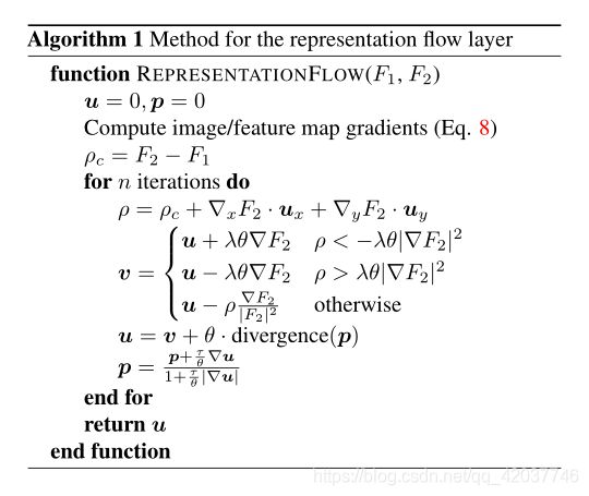
• CNN中的特征流 算法 1和图 2描述了我们特征流的过程。具有多个迭代的流层同样也可以共享参数（例如，图2中的每个蓝方框），每个层的表现取决于它先前的层。由于这个公式，层变得可微且允许学习所有参数，包括$(\tau ,\lambda ,\theta )$和散度权重$(w_x,w_y)$这使得我们的学习特征层可以为了其任务优化（比如行为识别）。

Computing Flow-of-Flow 计算Flow-of-Flow

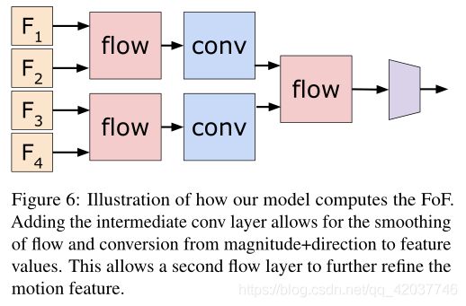
• Computing Flow-of-Flow Standard optical flow algorithms compute the flow for two sequential images. An optical flow image contains information about the direction and magnitude of the motion. Applying the flow algorithm directly on two flow images means that we are tracking pixels/locations showing similar motion in two consecutive frames. In practice, this typically leads to a worse performance due to inconsistent optical flow results and non-rigid motion. On the other hand, our representation flow layer is ‘learned’ from the data, and is able to suppress such inconsistency and better abstract/represent motion by having multiple regular convolutional layers between the flow layers. Fig. 6 illustrates such design, which we confirm its benefits in the experiment section. By stacking multiple representation flow layers, our model is able to capture longer temporal intervals and consider locations with motion consistency.
  
• 计算Flow-of-Flow 标准的光流算法计算两个序列图像的流。光流图像包含运动的方向和大小信息。直接运用硫酸法在两张流图上代表我们在连续两帧中展示跟踪像相似运动的素点/位置。在实际运动中，因为不一致的光流和非刚性的运动导致性能下降。另一个方面，我们的特征流层是从数据中学习的，能够在流层之间通过多次有规律的卷积来抑制不一致性和更好的抽象/表示运动。图 6展示了这个设计，实验证明了它的优势。通过叠加多个特征流层，我们的模型可以捕获更长时间范围并根据运动一致性确定位置。
• CNN feature maps may have hundreds or thousands of channels and our representation flow layer computes the flow for each channel, which can take significant time and memory. To address this, we apply a convolutional layer to reduce the number of channels from $C$ to $C^{{}^{\prime }}$ before the flow layer (note that $C^{{}^{\prime }}$ is still significantly more than traditional optical flow algorithms, which were only applied to single-channel, greyscale images). For numerical stability, we normalize this feature map to be in [0,255], matching standard image values. We found that the CNN features were quite small on average (< 0.5) and the TVL-1 algorithm default hyperparameters are designed for standard images values in [0,255], thus we found this normalization step important. Using the normalized feature, we compute the flow and stack the $x$ and $y$ flows, resulting in $2C^{{}^{\prime }}$channels. Finally, we apply another convolutional layer to convert from $2C^{{}^{\prime }}$ channels to $C$ channels. This is passed to the remaining CNN layers for the prediction. We average predictions from many frames to classify each video, as shown in Fig. 3.
  
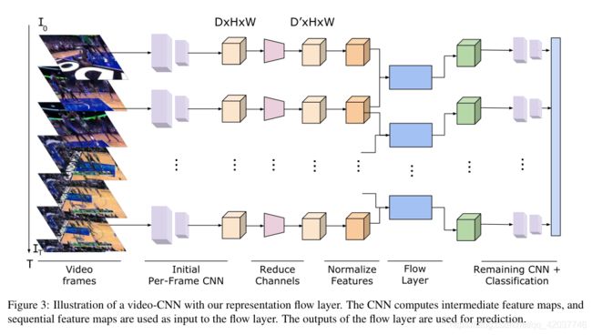
• CNN特征图有几百或者几千个通道，我们的特征流层计算每一个通道的流，这需要很多时间和存储空间。为了解决这个问题，我们运用一个卷积层来减少$C$到$C^{{}^{\prime }}$的通道的数（注意$C^{{}^{\prime }}$只应用于单通道灰度图像，但仍明显多于传统的光流算法）。为了数值稳定性，我们归一化特征图的大小为[0，255]，因此我们发现这个归一化步骤是重要的。使用归一化的特征，我们计算流并堆叠$x$$y$方向的流，产生$2C^{{}^{\prime }}$通道。最终，我们运用另一个卷积层转换$C$通道到$2C^{{}^{\prime }}$通道。这传递给剩下的CNN层进行预测。我们从很多帧来均值预测每个视频的类别，如图 3 所示。

3.3 Activity Recognition Model 行为识别模型

• We place the representation flow layer inside a standard activity recognition model taking a $T\times C\times W\times H$ tensor as input to a CNN. Here, $C$ is 3 as our model uses direct RGB frames as an input. $T$ is the number of frames the model processes, and $W$ and $H$ are the spatial dimensions. The CNN outputs a prediction per-timestep and these are temporally averaged to produce a probability for each class. The model is trained to minimize crossentropy:
  $$L(v,c)=-\sum (c==i)log(p_i)(11)$$
  where $p=M(v)$, $v$ is the video, the function $M$ is the classification CNN and $c$ represents which of the $K$ classes $v$ belongs. That is, the parameters in our flow layers are trained together with the other layers, so that it maximizes the final classification accuracy.
• 我们将特征流层放在一个标准的行为识别模型中，以$T\times C\times W\times H$的张量作为CNN的输入。这里，$C$是3，因为我们的模型采用RGB帧作为输入。$T$是模型处理的帧数，$W$和$H$是空间维度。CNN每一个时间段输出一个预测，去均值后产生每一类的概率。模型最小化交叉熵损失：
  $$L(v,c)=-\sum (c==i)log(p_i)(11)$$
  其中，$p=M(v)$，$v$是视频，函数$M$是分类CNN，$c$表示$v$属于$K$类中的一种。这也就是说，我们流层中的参数是和其他层一起训练的，从而使最后分类精度最高化。

4 Experiments 实验

Implementation details 实施细节

• Implementation details We implemented our representation flow layer in PyTorch and our code and models are available. As training CNNs on videos is computationally expensive, we used a subset of the Kinetics dataset [13] with 100k videos from 150 classes: Tiny-Kinetics. This allowed testing many models more quickly, while still having sufficient data to train large CNNs. For most experiments, we used ResNet-34 [10] with input of size $16\times 112\times 112$ (i.e., 16 frames with spatial size of 112). To further reduce the computation time for many studies, we used this smaller input, which reduces performance, but allowed us to use larger batch sizes and run many experiments more quickly. Our final models are trained on standard $224\times 224$ images. Check Appendix for specific training details.
• 实施细节 我们使用PyTorch来实施我们的特征流层，我们的代码和模型都是可用的。因为训练CNNs在视频上计算开销很小，我们使用Kinetics的一个来自于150个类包含100k个视频子集Tiny-Kinetics。这使得模型测试速度加快，同时也有足够的数据训练大的CNNs。对于大多数实验，我们使用输入尺寸为$16\times 112\times 112$的ResNet-34（例如，6帧尺寸为112）。为了更好的减少计算时间，我们使用更小的输入，这降低了性能，但允许我们使用更大的批处理大小和运行更多的实验。我们最终模型的是在$224\times 224$的图像上训练的。具体训练细节查看附录。

Where to compute flow? 在哪计算流？

• Where to compute flow? To determine where in the network to compute the flow, we compare applying our flow layer on the RGB input, after the first conv. layer, and after the each of the 5 residual blocks. The results are shown in Table 1. We find that computing the flow on the input provides poor performance, similar to the performance of the flow-only networks, but there is a significant jump after even 1 layer, suggesting that computing the flow of a feature is beneficial, capturing both the appearance and motion information. However, after 4 layers, the performance begins to decline as the spatial information is too abstracted/compressed (due to pooling and large spatial receptive field size), and sequential features become very similar, containing less motion information. Note that our HMDB performance in this table is quite low compared to state-of-the-art methods due to being trained from scratch using few frames and low spatial resolution ($112\times 112$). For the following experiments, unless otherwise noted, we apply the layer after the 3rd residual block. In Fig. 7, we visualize the learned motion representations computer after block 3.
  
  
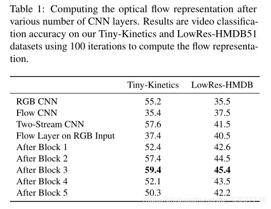
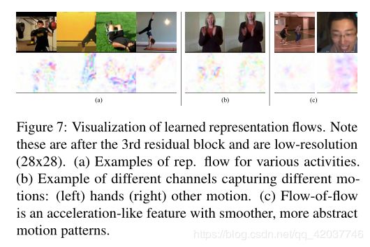
• 在哪里计算流？ 为决定在哪里计算流，我们将应用在RGB输入、第一个卷积层后和每五个残差模块后进行了比较。结果如表 1所示。我们发现在输入上计算流性能较差，接近仅流输入的网络，但在一层之后有显著的进步，这表明计算特征的流是有益的，可以捕获时间和运动信息。然后，在四层之后性能开始下降，因为空间信息太抽象/压缩（因为池化和空间感受野较大），序列图像变得很相似，包含的运动信息减少。注意与先进算法比较在HMDB上的性能表现差，这是因为开始训练的时候使用较少的帧和低的空间尺度（$112\times 112$）。在接下来的实验中，无特别说明，我们应用层在第三个残差模块后。在图 7中，我们可视化模块3之后的流运动特征计算。

What to learn? 学习什么？

• What to learn? As our method is fully differentiable, we can learn any of the parameters, such as the kernels used to compute image gradients, the kernels for the divergence computation and even $\tau$, $\lambda$, $\theta$. In Table 2, we compare the effects of learning different parameters. We find that learning the Sobel kernel values reduces performance due to noisy gradients particularly when the batch size is limited, but learning the divergence and $\tau$, $\lambda$, $\theta$ is beneficial.
  
• 学习什么 因为我们的方法是完全可微的，我们可以学习任何参数，比如计算图像梯度的核，计算散度的核以及$\tau$, $\lambda$, $\theta$。在表 2中，我们比较了学习不同参数的效果。我们发现Sobel核由于噪声梯度性能下降，尤其在批处理大小受限的时候，但是对于学习散度和$\tau$, $\lambda$, $\theta$是有益的。

How many iterations for flow? 需要迭代多少次？

• How many iterations for flow? To confirm that the iterations are important and determine how many we need, we experiment with various numbers of iterations. We compare the number of iterations needed for both learning ($divergence+\tau$, $\lambda$, $\theta$) and not learning parameters. The flow is computed after 3 residual blocks. The results are shown in Table 3. We find that learning provides better performance with fewer iterations (similar to the finding in [5]), and that iteratively computing the feature is important. We use 10 or 20 iterations in the remaining experiments as they provide good performance and are fast.
• 需要多少次迭代 为了证明迭代是重要，我们进行了不同数量的迭代操作。我们了比较学习($divergence+\tau$, $\lambda$, $\theta$)和非学习参数所需要的迭代次数。流是在第三个残差模块后计算。结果展示在表 3中。我们发现采用更少的迭代的学习可以提高更好的性能（同[5]中的发现），也说明迭代计算特征是重要的。我们采用10或者20次迭代在其余实验中，因为他们提供了好的性能和速度。

Two-stream fusion? 双流融合？

• Two-stream fusion? Two-stream CNNs fusing both RGB and optical flow features has been heavily studied [20, 7]. Based on these works, we compare various ways of fusing RGB and our flow representation, shown in Fig. 4. We compare no fusion, late fusion (i.e., separate RGB and flow CNNs) and addition/multiplication/concatenation fusion. In Table 4, we compare different fusion methods for different locations in the network. We find that fusing RGB information is very important “when computing flow directly from RGB input”. However, it is not as beneficial when computing the flow of representations as the CNN has already abstracted much appearance information away. We found that concatenation of the RGB and flow features perform poorly compared to the others. We do not use two-stream fusion in any other experiments, as we found that computing the representation flow after the 3rd residual block provides sufficient performance even without any fusion.
  
  
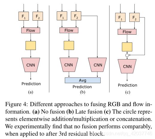
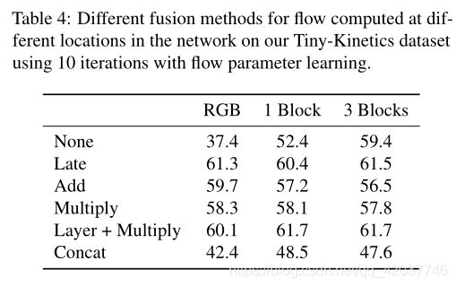
• 双流融合？ 将RGB和光流特征融合的双流CNNs已经进行了大量的研究。在这些工作的基础上，我们比较了各种RGB融合和我们的流特征，结果在图 4中展示。我们比较了无融合、晚期融合（比如，分开的RGB和流CNNs）以及加法/乘法/连接融合。在表 4中，我们比较不同位置的不同融合方法。我们发现 “直接从RGB输入计算流” 时融合RGB信息非常重要。然而，这在计算特征流不那么有用，因为CNN已经获取了很多外观信息。我们发现连接RGB和流特征的性能比其他方法要差。我们不使用双流融合在其他实验中，因为我们发现及时没有任何融合在第三个残差模块后计算流特征性能也不错。

Flow-of-flow Flow-of-flow

• Flow-of-flow We can stack our layer multiple times, computing the flow-of-flow (FoF). This has the advantage of combining more temporal information into a single feature. Our results are shown in Table 5. Applying the TV-L1 algorithm twice gives quite poor performance, as optical flow features do not really satisfy the brightness consistency assumption, as they capture magnitude and direction of motion (shown in Fig. 5). Applying our representation flow layer twice performs significantly better than TV-L1 twice, but still worse than our baseline of not doing so. However, we can add a convolutional layer between the first and second flow layer, flow-conv-flow (FcF), (Fig. 6), allowing the model to better learn longer-term flow representations. We find this performs best, as this intermediate layer is able to smooth the flow and produce a better input for the representation flow layer. However, we find adding a third flow layer reduces performance as the motion representation becomes unreliable, due to the large spatial receptive field size. In Fig. 7, we visualize the learned flow-of-flow, which is a smoother, acceleration-like feature with abstract motion patterns.
  
  
  
  
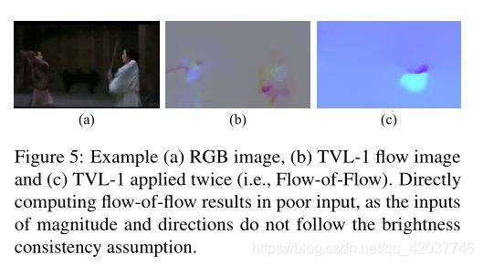
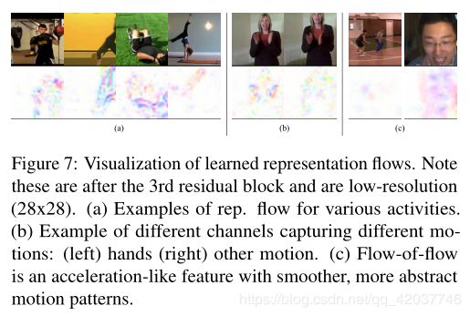
• Flow-of-flow 我们可以多次叠加我们的层，计算flow-of-flow(FoF)。这样做的好处是将更多的时间信息结合到单个特征中。我们的结果在表 5中展示。两次使用TV-L1的表现很差，因为光流特征捕获运动的大小和方向时难以满足亮度一致性假设（如图 5所示）。两次使用我们的特征流层性能比TV-L1好，但是仍然比不使用的基准性能差。然后，我们在第一个和第二个流层之间增加一个卷积层，flow-conv-flow (FcF)（图 6），允许模型更好的学习长时间范围的六特征。我们发现这个表现最好，因为这个中间层可以平滑两个流层且为特征流层产生更好的输入。然而，我们发现添加第三个流层降低了性能，因为空间感受野较大运动特征开始变得不可靠。在图 7中，我们可视化更平滑、类似加速特征的flow-of-flow。

Flow of 3D CNN Feature 3D CNN的流

• Flow of 3D CNN Feature Since 3D convolutions capture some temporal information, we test computing our flow representation on features from a 3D CNN. As 3D CNNs are expensive to train, we follow the method of I3D [3] to inflate a ResNet-18 pretrained on ImageNet to a 3D CNN for videos. We also compare to the (2+1)D method of spatial conv. followed by temporal conv from [26], which produces a similar feature combining spatial and temporal information. We find our flow layer increases performance even with 3D and (2+1)D CNNs already capturing some temporal information: Tables 6 and 7. These experiments used 10 iterations and learning the flow parameters. In these experiments, FcF was not used.
• 由于3D卷积不活了一些时间信息，我们在3D CNN上测试计算流特征图。因为3D CNNs难以训练，我们采用I3D方法，将在ResNet-18上预训练的图像扩展到用于视频的3D CNN。我们也比较了空间卷积的(2+1)D方法，然后从[26]中提取时间序列，得到了结合时空信息的相似特征。我们发现我们的流层提高了性能，即使3D和（2+1）D CNNs已经获得了一些时间信息：表 6和7。这些实验使用了10次迭代来学习流参数，FcF未被使用。
• We also compared to the OFF [21] using (2+1)D and 3D CNNs. We observe that this method does not result in meaningful performance increases using CNNs that capture temporal information, while our approach does.
• 我们还使用(2+1)D和3D cnn与OFF[21]进行了比较。观察发现使用CNNs捕获时间信息并没有使得性能得到有效提升，但我们的方法可以。

Comparison to other motion representations 与其他运动特征进行比较

• Comparison to other motion representations We compare to existing CNN-based motion representation methods to confirm the usefulness of our representation flow. For these experiments, when available, we used code provided by the authors and otherwise implemented the methods ourselves. To better compare to existing works, we used $(16\times )224\times 224$ images. Table 8 shows the results. MFNet [15] captures motion by spatially shifting CNN feature maps, then summing the results, TVNet [5] applies a convolutional optical flow method to RGB inputs, and ActionFlowNet [16] trains a CNN to jointly predict optical flow and activity classes. We also compare to OFF [21] using only RGB inputs. Note that the HMDB performance in [21] was reported using their three-stream model (i.e., RGB + RGB-diff + optical flow inputs), and here we compare to the version only using RGB. Our method, which applies the iterative flow computation on CNN feature maps, performs the best.
  
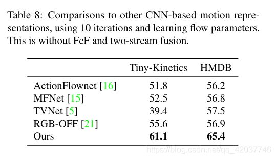
• 与其他运动特征进行比较 我们与现存的以CNN为基础的运动特征方法比较，证明了我们的特征流是有用的。对于这些实验，我们使用了作者提供的代码或者用自己的方法实现。为了更好的与现有的工作比较，我们使用$(16\times )224\times 224$尺寸的图像。表 8展示了结果。MFNet [15]通过空间移动的CNN特征图捕获运动，然后将结果相加；TVNet [5]对RGB输入使用卷积光流方法；ActionFlowNet [16]训练一个CNN联合预测光流和行为分类。我们也与仅RGB为输入的OFF进行比较。注意到[21]在HMDB上的性能是在使用三流模型得到的（即，RGB+RGB差异+光流输入），这里我们与仅使用RGB输入比较。我们的方法在CNN feature map上应用迭代流计算，效果最好。

Computation time 计算时间

• Computation time We compare our representation flow to state-of-the-art two-stream approaches in terms of run-time and number of parameters. All timings were measured using a single Pascal Titan X GPU, for a batch of videos with size $32\times 224\times 224$. The flow/two-stream CNNs include the time to run the TV-L1 algorithm (OpenCV GPU version) to compute the optical flow. All CNNs were based on the ResNet-34 architecture. As also shown in Table 9, our method is significantly faster than two-stream models relying on TV-L1 or other optical flow methods, while performing similarly or better. The number of parameters our model has is half of its two-stream competitors (e.g., 21M vs. 42M, in the case of 2D CNNs).
• 计算时间 我们将我们的特征流方法与先进的双流方法就运行时间和参数数量进行比较。所有的时间是在使用单个Pascal Titan X GPU处理批处理大小为$32\times 224\times 224$的视频上计算的。流/双流CNNs包含运行TV-L1（OpenCV GPU 版本）计算光流的时间。所有CNNs是以ResNet-34为基础架构。如表 9所示，我们的方法比依赖TV-L1的双流模型或者其他光流模型更快，而且性能相似甚至更好。我们模型的参数是双流模型的一半（例如，在2D CNNs中，是2100百万与4200百万）。

Comparison to state-of-the-arts 与先进算法进行比较

• Comparison to state-of-the-arts We also compared our action recognition accuracies with the state-of-the-arts on Kinetics and HMDB. For this, we train our models using $32\times 224\times 224$ inputs with the full kinetics dataset, using 8 V100s. We used the 2D ResNet-50 as the architecture. Based on our experiments, we applied our representation flow layer after the 3rd residual block, learned the hyperparameters and divergence kernels, and used 20 iterations. We also compare our flow-of-flow model. Following [22], the evaluation is performed using a running average of the parameters over time. Our results, shown in Table 9, confirm that this approach clearly outperforms existing models using RGB only inputs, and is competitive against expensive two-stream networks. Our model performs the best among those not using optical flow inputs (i.e., among the models only taking ∼600ms per video). The models requiring optical flow were more than 10 times slower, including two-stream versions of [3, 25, 26]
  
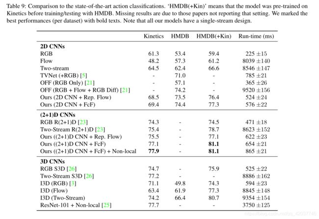
• 与先进算法进行比较 我们将我们的算法与其他先进的算法在Kinetics和HMDB数据集上进行了比较。为此，我们使用尺寸为$32\times 224\times 224$作为输入在全Kinetics数据集上来训练我们的模型。我们使用2D ResNet-50作为架构。在我们实验的基础上，我们将特征流层应用在第三个残差模块之后，使用20个迭代学习超参数和散度核。我们同样与flow-of-flow模型比较。在[22]之后，使用参数随时间的运行均值来评估。我们的结果在表 9 中展示，证实了这个方法的性能比现存的仅使用RGB作为输入的模型好，而且比计算开销大的双流网络更有竞争力。我们的模型在不使用光流输入中性能最好（在这些模型中仅使用600ms的视频）需要光流的模型慢10倍以上，包括双流模型[3, 25, 26]

5 Conclusion 结论

• We introduced a learnable representation flow layer in- spired by optical flow algorithms. We experimentally compared various forms of our layer to confirm that the iterative optimization and learnable parameters are important. Our model clearly outperformed existing methods in both speed and accuracy on standard datasets. We also introduced the concept of ‘flow of flow’ to compute longer-term motion representations and showed it benefits performance.
• 我们介绍了一种基于光流法启发的可学习特征流层。我们通过实验比较了我们层的各种形式，证明了迭代优化和可学习参数是重要的。我们的模型在标准数据集上的速度和精度的表现明显好于现存方法。我们也介绍了‘flow of flow’的概念去计算长时间运动特征，并展示了它的优秀性能。

"
一些方法与代码还未理解、研究，等待后续补充。
"