Kaggle: Tweet Sentiment Extraction 方法总结 Part 1/2: 常用方法总结
文章目录
- 往期文章目录链接
- Note
- Before we start
- Tweet Sentiment Extraction
- What is the MAGIC?
- Common Methods
- Label Smoothing
- Implementation of Label Smoothing
- In tensorflow
- In pytorch
- Multi-sample dropout
- Implementation
- Stochastic Weight Averaging (SWA)
- Different learning rate settings for encoder and head
- Customized Layer Initialization
- 往期文章目录链接
往期文章目录链接
Note
This post is the first part of overall summarization of the competition. The second half is here.
Before we start
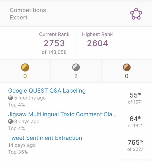
I attended two NLP competition in June, Tweet Sentiment Extraction and Jigsaw Multilingual Toxic Comment Classification, and I’m happy to be a Kaggle Expert from now on
Tweet Sentiment Extraction
Goal:
The objective in this competition is to “Extract support phrases for sentiment labels”. More precisely, this competition asks kagglers to construct a model that can figure out what word or phrase best supports the given tweet from the labeled sentiment. In other word, kagglers’re attempting to predict the word or phrase from the tweet that exemplifies the provided sentiment. The word or phrase should include all characters within that span (i.e. including commas, spaces, etc).
For example:
text         : "Sooo SAD I will miss you here in San Diego!!!"
sentiment    : negative
selected_text: "Sooo SAD"
In this competition, the state-of-the-art (SOTA) transformer models were not so bad in extracting the selected_text. The main problem was to capture the “noise” in the dataset.
The organizer of this competition did not introduce the “noise” (magic of the competition) on purpose but probably by some regex mistake (I’ll talk about the “noise” in the next section). When I analyzed the data, I found some weird selected_text like most other teams did. For example,
text         : "  ROFLMAO for the funny web portal  =D"
sentiment    : positive
selected_text: "e funny"
---------------------------------------------------------------
text         : " yea i just got outta one too....i want him
                 back tho  but i feel the same way...i`m cool
                 on dudes for a lil while"
sentiment    : positive
selected_text: "m cool"
However, most teams (including my team) did not strive to figure out how such weird selected_text are selected or just treated it as a mistake such that they chose to ignore it in the consideration of overfitting if trying to correct it.
This turns out to be a watershed of this competition. Teams solved this problem were still among the top ranked positions in the private leaderboard but those who did not fix this problem had shakes on their ranks to some degree. I found that the scores of top 30 30 30 teams are mostly stable but other than those, the private LB had a huge shake that was out of my expectation. The fun part is: I know there would be a shake in the competition, so I gave my team the name Hope no shake, but it didn’t help at all . My team was in the silver medal range in the public LB but our rank dropped to almost 800 800 800th in the private LB! What a shame! There are teams even more unfortunate than us and dropped their ranks from top 50 to bottom 200…
Anyway, there are still some fancy and interesting solution among top ranked teams and their solutions can be divided into three categories:
- Solution with character-level model only (First place solution! Awesome!).
- solution with well-designed post-processing.
- Bolution with both character-level model and well-designed post-processing.
After the competition, I spend one week trying to understand their solutions and unique ideas and really learned a lot. So here I would like to share their ideas to those who are interested.
In the rest of the post, I made a summary of the top solutions and also add some of my understanding. The reference are at the bottom. So let’s get started!
What is the MAGIC?
This is just a bug introduced when the competition holder created this task. Here shows a representative example and we call this the “noise” in the labels.
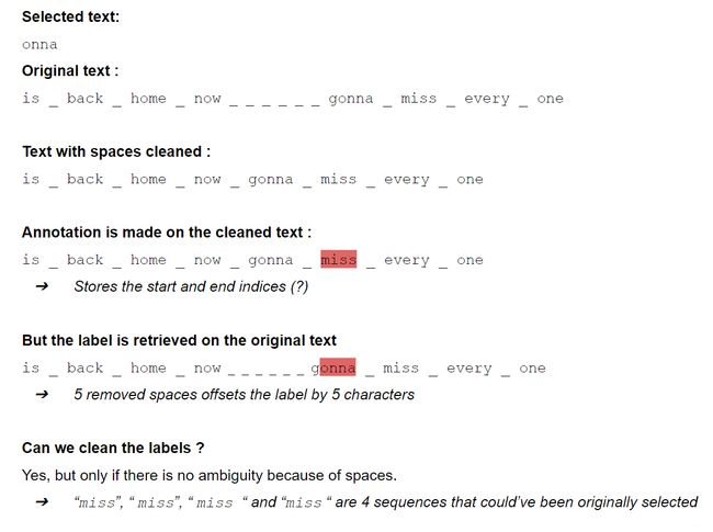
The given original annotation is “onna” but it is too weird. The true annotation should be “miss” (this is a negative sentence). We think that the host applied a wrong slice obtained on the normalized text without consequence spaces for the original text with plenty of spaces, emojis, or emoticons.
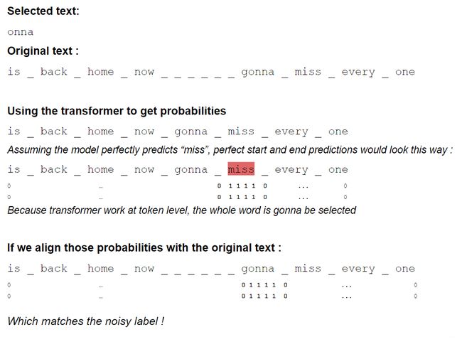
Here is how to solve it theoretically:
- Recover true annotation from the buggy annotation (pre-processing).
- Train model with true annotation.
- Predict the right annotation.
- Project back the right annotation to the buggy annotation (post-processing).
Here is the visualization:
Common Methods
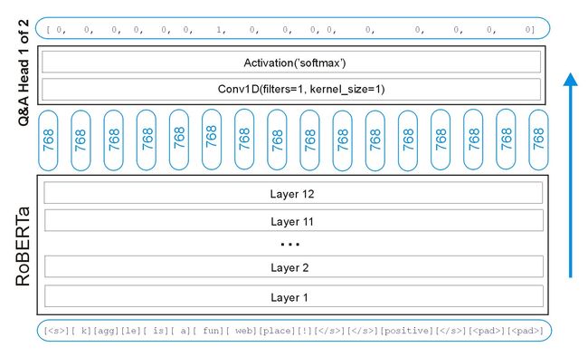
Most Kagglers use the following model structure (from public notebook) as a baseline and here is the illustration (I copied it from the author, the link in at the bottom of the post). This is the tensorflow version:
We are given text, selected_text, and sentiment. For roBERTa model, we prepare question answer as text sentiment
After converting text and selected_text into tokens, we can then determine the start index and end index of selected_text within text. We will one hot encode these indices. Below are the required inputs and targets for roBERTa. In this example, we have chosen roBERTa with max_len=16, so our input_ids have 2

We begin with vanilla TFRobertaModel. This model takes our 16 (max_len) input_ids and outputs 16 16 16 vectors each of length 768. Each vector is a representation of one input token.
We then apply tf.keras.layers.Conv1D(filters=1, kernel_size=1) which transforms this matrix of size ( 768 , 16 768, 16 768,16) into a vector of size (1, 16). Next we apply softmax to this length 16 16 16 vector and get a one hot encoding of our start_index. We build another head for our end_index.
Most top ranked kagglers implemented the following two methods: Label Smoothing and Multi-sample Dropout. SO I would like to talk about this methods first before I go forward.
Label Smoothing
When we apply the cross-entropy loss to a classification task, we’re expecting true labels to have 1, while the others 0. In other words, we have no doubts that the true labels are true, and the others are not. Is that always true in our case? As a result, the ground truth labels we have had perfect beliefs on are possibly wrong.
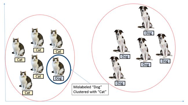
One possible solution to this is to relax our confidence on the labels. For instance, we can slightly lower the loss target values from 1 to, say, 0.9. And naturally, we increase the target value of 0 for the others slightly as such. This idea is called label smoothing.
The smoothed labels are calculated by
new_onehot_labels = onehot_labels * (1 – label_smoothing) + label_smoothing / num_classes
Foe example, suppose we are training a model for binary classification, and our labels are 0 0 0 for Non-toxic, 1 1 1 for toxic. Now, say you set label_smoothing = 0.2, then using the equation above, we get:
new_labels = [0, 1] * (1 — 0.2) + 0.2 / 2 = [0, 1]*(0.8) + 0.1 = [0.1 ,0.9]
Implementation of Label Smoothing
In tensorflow
tf.keras.losses.binary_crossentropy(
    y_true, y_pred,
    from_logits=False,
    label_smoothing=0
)
In pytorch
There are multiple ways to achieve this, I list two here.
- way 1
class LabelSmoothing(nn.Module):
    def __init__(self, smoothing = 0.1):
        super(LabelSmoothing, self).__init__()
        self.confidence = 1.0 - smoothing
        self.smoothing = smoothing

    def forward(self, x, target):
        if self.training:
            x = x.float()
            target = target.float()
            logprobs = torch.nn.functional.log_softmax(x, dim = -1)
            nll_loss = -logprobs * target
            nll_loss = nll_loss.sum(-1)
            smooth_loss = -logprobs.mean(dim=-1)
            loss = self.confidence * nll_loss + self.smoothing * smooth_loss
            return loss.mean()
        else:
            return torch.nn.functional.cross_entropy(x, target)
Somehow in the training step, you would use label smoothing like this:
criterion = LabelSmoothing()
loss = criterion(outputs, targets)
- way 2
class LabelSmoothing(nn.Module):
    def __init__(self, classes, smoothing=0.0, dim=-1):
        super(LabelSmoothing, self).__init__()
        self.confidence = 1.0 - smoothing
        self.smoothing = smoothing
        self.cls = classes
        self.dim = dim

    def forward(self, pred, target):
        pred = pred.log_softmax(dim=self.dim)
        with torch.no_grad():
            # true_dist = pred.data.clone()
            true_dist = torch.zeros_like(pred)
            true_dist.fill_(self.smoothing / (self.cls - 1))
            true_dist.scatter_(1, target.data.unsqueeze(1), self.confidence)
        return torch.mean(torch.sum(-true_dist * pred, dim=self.dim))
Multi-sample dropout
This is also an idea from the 1st place solution of the last competition I attended (Google QUEST Q&A Labeling). The idea came from a paper called Multi-Sample Dropout for Accelerated Training and Better Generalization.
The original dropout creates a randomly selected subset (called a dropout sample) from the input in each training iteration while the multi-sample dropout creates multiple dropout samples. The loss is calculated for each sample, and then the sample losses are averaged to obtain the final loss. Experimental results showed that multi-sample dropout significantly accelerates training by reducing the number of iterations until convergence Experiments also showed that networks trained using multi-sample dropout achieved lower error rates and losses for both the training set and validation set.
Implementation
The implementation is not that hard and the following is part of my code used in the competition.
def forward(self, input_ids, attention_mask):

    # `hs` is the 12 hidden layers. Later we uses hs[-1], hs[-2]
    # which are the last 2 hidden layers. batch_size=16.
    _, _, hs = self.roberta(input_ids, attention_mask)

#     x = torch.stack([hs[-1], hs[-2]])   # torch.Size([2, 16, 96, 768])
#     x = x[0] * 0.9 + x[1] * 0.1         # torch.Size([16, 96, 768])

    stacked = torch.stack([hs[-1], hs[-2]])    # torch.Size([2, 16, 96, 768])
    apool= torch.mean(stacked, 0)              # torch.Size([16, 96, 768])
    mpool, _ = torch.max(stacked, 0)           # torch.Size([16, 96, 768])
    x = torch.cat((apool, mpool), -1)          # torch.Size([16, 96, 768 * 2])

    # Multisample Dropout: https://arxiv.org/abs/1905.09788
    logits = torch.mean(
        torch.stack(
            [self.fc(self.high_dropout(x)) for _ in range(5)],
            dim=0,
        ),
        dim=0,
    )

    start_logits, end_logits = logits.split(1, dim=-1)    # torch.Size([16, 96, 1])
    start_logits = start_logits.squeeze(-1)               # torch.Size([16, 96])
    end_logits = end_logits.squeeze(-1)                   # torch.Size([16, 96])

    return start_logits, end_logits
Stochastic Weight Averaging (SWA)
Author: by Pavel Izmailov and Andrew Gordon Wilson
Stochastic Weight Averaging (SWA) is a simple procedure that improves generalization in deep learning over Stochastic Gradient Descent (SGD) at no additional cost, and can be used as a drop-in replacement for any other optimizer in PyTorch.
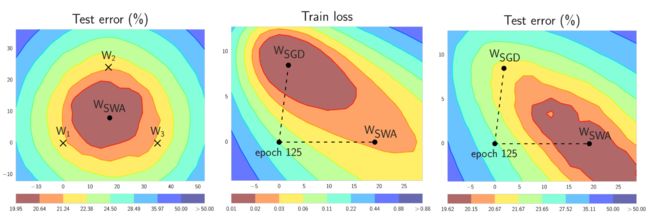
In short, SWA performs an equal average of the weights traversed by SGD with a modified learning rate schedule. SWA solutions end up in the center of a wide flat region of loss, while SGD tends to converge to the boundary of the low-loss region, making it susceptible to the shift between train and test error surfaces (see the middle and right panels in the figure below):
With the implementation in torchcontrib, using SWA is as easy as using any other optimizer in PyTorch:
from torchcontrib.optim import SWA
# training loop
base_opt = torch.optim.SGD(model.parameters(), lr=0.1)
opt = torchcontrib.optim.SWA(base_opt, swa_start=10, swa_freq=5, swa_lr=0.05)
for _ in range(100):
     opt.zero_grad()
     loss_fn(model(input), target).backward()
     opt.step()
opt.swap_swa_sgd()
You can wrap any optimizer from torch.optim using the SWA class, and then train your model as usual. When training is complete you simply call swap_swa_sgd() to set the weights of your model to their SWA averages. Below we explain the SWA procedure and the parameters of the SWA class in detail. We emphasize that SWA can be combined with any optimization procedure, such as Adam, in the same way that it can be combined with SGD.
For the following methods, we assume that we are writing a customized roberta model and here is the beginning of the customized roberta class
class CustomRoberta(nn.Module):

    def __init__(self, path='path/to/roberta-base/pytorch_model.bin'):
        super(CustomRoberta, self).__init__()

        config = RobertaConfig.from_pretrained(
            'path/to/roberta-base/config.json', output_hidden_states=True)

        self.roberta = RobertaModel.from_pretrained(path, config=config)
        self.weights_init_custom()

    # ignore the detail
    def forward(*args):
        pass
Different learning rate settings for encoder and head
This is an idea from the last competition I attended called Google QUEST Q&A Labeling, and this idea is mentioned in the 1st place solution.
param_optimizer = list(model.named_parameters())
no_decay = ['bias', 'LayerNorm.bias', 'LayerNorm.weight']
optimizer_grouped_parameters = [
    {'params': [p for n, p in param_optimizer if not any(nd in n for nd in no_decay)], 'weight_decay': 0.01},
    {'params': [p for n, p in param_optimizer if any(nd in n for nd in no_decay)], 'weight_decay': 0.0}
   ]

num_train_optimization_steps = int(EPOCHS*len(train_df)/batch_size/accumulation_steps)

optimizer = AdamW(optimizer_grouped_parameters, lr=lr, correct_bias=False)

scheduler1 = get_linear_schedule_with_warmup(optimizer, num_warmup_steps=0.1*num_train_optimization_steps, num_training_steps=num_train_optimization_steps)
scheduler2 = get_constant_schedule(optimizer)
Customized Layer Initialization
The following code is an initialization of the last three layers of the model.
def weights_init_custom(self):
    init_layers = [9, 10, 11]
    dense_names = ["query", "key", "value", "dense"]
    layernorm_names = ["LayerNorm"]
    for name, module in self.roberta.named_parameters():
        if any(f".{i}." in name for i in init_layers):
            if any(n in name for n in dense_names):
                if "bias" in name:
                    module.data.zero_()
                elif "weight" in name:
                    module.data.normal_(mean=0.0, std=0.02)
            elif any(n in name for n in layernorm_names):
                if "bias" in name:
                        module.data.zero_()
                elif "weight" in name:
                    module.data.fill_(1.0)
Let’s break it into parts. Let’s see an example of a pair of name and module in self.roberta.named_parameters():
>>> name, module
('embeddings.word_embeddings.weight', Parameter containing:
 tensor([[ 0.1476, -0.0365,  0.0753,  ..., -0.0023,  0.0172, -0.0016],
         [ 0.0156,  0.0076, -0.0118,  ..., -0.0022,  0.0081, -0.0156],
         [-0.0347, -0.0873, -0.0180,  ...,  0.1174, -0.0098, -0.0355],
         ...,
         [ 0.0304,  0.0504, -0.0307,  ...,  0.0377,  0.0096,  0.0084],
         [ 0.0623, -0.0596,  0.0307,  ..., -0.0920,  0.1080, -0.0183],
         [ 0.1259, -0.0145,  0.0332,  ...,  0.0121,  0.0342,  0.0168]],
        requires_grad=True))
The followings are some examples of weights in the last three layers that they want to initialize:
encoder.layer.9.attention.self.query.weight
encoder.layer.9.attention.self.query.bias
encoder.layer.9.attention.self.key.weight
encoder.layer.9.attention.self.key.bias
encoder.layer.9.attention.self.value.weight
encoder.layer.9.attention.self.value.bias
encoder.layer.9.attention.output.dense.weight
encoder.layer.9.attention.output.dense.bias
encoder.layer.9.attention.output.LayerNorm.weight
encoder.layer.9.attention.output.LayerNorm.bias
Reference:
- 1st place solution: https://www.kaggle.com/c/tweet-sentiment-extraction/discussion/159254
- 1st place solution code: https://www.kaggle.com/theoviel/character-level-model-magic
- 2nd place solution: https://www.kaggle.com/c/tweet-sentiment-extraction/discussion/159310
- 2nd place solution code: https://www.kaggle.com/hiromoon166/inference-8models-seed100101-bucketing-2-ver2/input?select=pre_processed.txt#Inference-of-Reranking-model
- 2nd place post-processing: https://www.kaggle.com/futureboykid/2nd-place-post-processing
- 3rd place solution: https://www.kaggle.com/c/tweet-sentiment-extraction/discussion/159910
- 3rd place solution code: https://github.com/suicao/tweet-extraction
- 4th place solution: https://www.kaggle.com/c/tweet-sentiment-extraction/discussion/159499
- 5th place solution: https://www.kaggle.com/c/tweet-sentiment-extraction/discussion/159268
- Label Smoothing code: https://www.kaggle.com/shonenkov/tpu-training-super-fast-xlmroberta, https://github.com/pytorch/pytorch/issues/7455
- Label Smoothing: https://www.flixstock.com/label-smoothing-an-ingredient-of-higher-model-accuracy, https://www.kaggle.com/shahules/tackle-with-label-smoothing-proved
- Multi-Sample Dropout for Accelerated Training and Better Generalization: https://arxiv.org/pdf/1905.09788.pdf
- https://stackoverflow.com/questions/50747947/embedding-in-pytorch
- sequence-bucketing: https://www.kaggle.com/bminixhofer/speed-up-your-rnn-with-sequence-bucketing#Implementation-&-comparing-static-padding-with-sequence-bucketing
- Re-ranking in QA paper: https://arxiv.org/pdf/1906.03008.pdf
- Common model structure: https://www.kaggle.com/c/tweet-sentiment-extraction/discussion/143281
- SWA: https://pytorch.org/blog/stochastic-weight-averaging-in-pytorch/