【计算机视觉】图像全景拼接 RANSAC

1、全景图像拼接原理

1.1 RANSAC算法原理

RANSAC是“RANdom SAmple Consensus（随机抽样一致）”的缩写。它可以从一组包含“局外点”的观测数据集中，通过迭代方式估计数学模型的参数。它是一种不确定的算法——它有一定的概率得出一个合理的结果；为了提高概率必须提高迭代次数。

RANSAC的基本假设是：

（1）数据由“局内点”组成，例如：数据的分布可以用一些模型参数来解释；

（2）“局外点”是不能适应该模型的数据；

（3）除此之外的数据属于噪声。

局外点产生的原因有：噪声的极值；错误的测量方法；对数据的错误假设。

RANSAC也做了以下假设：给定一组（通常很小的）局内点，存在一个可以估计模型参数的过程；而该模型能够解释或者适用于局内点。

RANSAC的算法步骤：

   1. 随机从数据集中随机抽出4个样本数据 (此4个样本之间不能共线)，计算出变换矩阵H，记为模型M；

   2. 计算数据集中所有数据与模型M的投影误差，若误差小于阈值，加入内点集 I

   3. 如果当前内点集 I 元素个数大于最优内点集 I_best , 则更新 I_best = I，同时更新迭代次数k ;

   4. 如果迭代次数大于k,则退出 ; 否则迭代次数加1，并重复上述步骤；

  注：迭代次数k在不大于最大迭代次数的情况下，是在不断更新而不是固定的

  其中，p为置信度，一般取0.995；w为"内点"的比例 ; m为计算模型所需要的最少样本数=4；

1.2 单应性矩阵估计

平面的单应性被定义为一个平面到另外一个平面的投影映射。

这边通过ransac算法来求解单应性矩阵。

1.3 图像拼接

  使用RANSAC算法估计出图像间的单应性矩阵，将所有的图像扭曲到一个公共的图像平面上。通常，这里的公共平面为中心图像平面。一种方法是创建一个很大的图像，比如将图像中全部填充0，使其和中心图像平行，然后将所有的图像扭曲到上面。由于我们所有的图像是由照相机水平旋转拍摄的，因此我们可以使用一个较简单的步骤：将中心图像左边或者右边的区域填充为0，以便为扭曲的图像腾出空间。

2、图像拼接代码实现

 使用RANSAC算法求解单应性矩阵 RansacModel类是用于测试单应性矩阵的类 里面包含了fit（）和get_error()方法

fit()方法计算选取的四个对应的单应性矩阵

get_error() 是对所有的对应计算单应性矩阵，然后对每个变换后的点，返回相应的误差

class RansacModel(object):
    """ Class for testing homography fit with ransac.py from
        http://www.scipy.org/Cookbook/RANSAC"""

    def __init__(self, debug=False):
        self.debug = debug

    def fit(self, data):
        """ Fit homography to four selected correspondences. """

        # transpose to fit H_from_points()
        data = data.T

        # from points
        fp = data[:3, :4]
        # target points
        tp = data[3:, :4]

        # fit homography and return
        return H_from_points(fp, tp)

    def get_error(self, data, H):
        """ Apply homography to all correspondences,
            return error for each transformed point. """

        data = data.T

        # from points
        fp = data[:3]
        # target points
        tp = data[3:]

        # transform fp
        fp_transformed = dot(H, fp)

        # normalize hom. coordinates
        for i in range(3):
            fp_transformed[i]/=fp_transformed[2]

        # return error per point
        return sqrt(sum((tp - fp_transformed) ** 2, axis=0))

H_from_ransac() 使用RANSAC稳健性估计点对应间的单应性矩阵H。该函数允许提供阈值和最小期望的点对数目。最重要的参数是最大迭代次数：程序退出太早可能得到一个坏解；迭代次数太多会占有太多时间。函数的返回结果为单应性矩阵和对应该单应性矩阵的正确点对。

def H_from_ransac(fp, tp, model, maxiter=1000, match_theshold=10):
    """ Robust estimation of homography H from point
        correspondences using RANSAC (ransac.py from
        http://www.scipy.org/Cookbook/RANSAC).

        input: fp,tp (3*n arrays) points in hom. coordinates. """

    import ransac

    # group corresponding points
    data = vstack((fp, tp))

    # compute H and return
    H, ransac_data = ransac.ransac(data.T, model, 4, maxiter, match_theshold, 10, return_all=True)
    return H, ransac_data['inliers']

  拼接图像 panorama（）使用单应性矩阵H（使用RANSAC健壮性估计得出），协调两幅图像，创建水平全景图像。结果为一幅和toim具有相同高度的图像。padding指定填充像素的数目，delta指定额外的平移量。对于通用的geometric_transform()函数，我们需指定能够描述像素到像素间映射的函数。此例子中，transf（）函数就是该指定的函数。该函数通过将像素和H相乘，然后对齐次坐标进行归一化来实现像素间的映射。通过查看H中的平移量我们可以决定应该将图像填补到左边还是右边。当该图像填补到左边时，由于目标图像中的点坐标也变化了，

def panorama(H, fromim, toim, padding=2400, delta=2400):
    """ Create horizontal panorama by blending two images
        using a homography H (preferably estimated using RANSAC).
        The result is an image with the same height as toim. 'padding'
        specifies number of fill pixels and 'delta' additional translation. """

    # check if images are grayscale or color
    is_color = len(fromim.shape) == 3

    # homography transformation for geometric_transform()
    def transf(p):
        p2 = dot(H, [p[0], p[1], 1])
        return (p2[0] / p2[2], p2[1] / p2[2])

    if H[1, 2] < 0:  # fromim is to the right
        print('warp - right')
        # transform fromim
        if is_color:
            # pad the destination image with zeros to the right
            toim_t = hstack((toim, zeros((toim.shape[0], padding, 3))))
            fromim_t = zeros((toim.shape[0], toim.shape[1] + padding, toim.shape[2]))
            for col in range(3):
                fromim_t[:, :, col] = ndimage.geometric_transform(fromim[:, :, col],
                                                                  transf, (toim.shape[0], toim.shape[1] + padding))
        else:
            # pad the destination image with zeros to the right
            toim_t = hstack((toim, zeros((toim.shape[0], padding))))
            fromim_t = ndimage.geometric_transform(fromim, transf,
                                                   (toim.shape[0], toim.shape[1] + padding))
    else:
        print('warp - left')
        # add translation to compensate for padding to the left
        H_delta = array([[1, 0, 0], [0, 1, -delta], [0, 0, 1]])
        H = dot(H, H_delta)
        # transform fromim
        if is_color:
            # pad the destination image with zeros to the left
            toim_t = hstack((zeros((toim.shape[0], padding, 3)), toim))
            fromim_t = zeros((toim.shape[0], toim.shape[1] + padding, toim.shape[2]))
            for col in range(3):
                fromim_t[:, :, col] = ndimage.geometric_transform(fromim[:, :, col],
                                                                  transf, (toim.shape[0], toim.shape[1] + padding))
        else:
            # pad the destination image with zeros to the left
            toim_t = hstack((zeros((toim.shape[0], padding)), toim))
            fromim_t = ndimage.geometric_transform(fromim,
                                                   transf, (toim.shape[0], toim.shape[1] + padding))

    # blend and return (put fromim above toim)
    if is_color:
        # all non black pixels
        alpha = ((fromim_t[:, :, 0] * fromim_t[:, :, 1] * fromim_t[:, :, 2]) > 0)
        for col in range(3):
            toim_t[:, :, col] = fromim_t[:, :, col] * alpha + toim_t[:, :, col] * (1 - alpha)
    else:
        alpha = (fromim_t > 0)
        toim_t = fromim_t * alpha + toim_t * (1 - alpha)

    return toim_t

主文件

先使用SIFT特征自动找到匹配对应。

from pylab import *
from PIL import Image
import warp
import homography
import sift

# set paths to data folder
featname = ['image/' + str(i + 1) + '.sift' for i in range(3)]
imname = ['image/' + str(i + 1) + '.jpg' for i in range(3)]

# extract features and match
l = {}
d = {}
for i in range(3):
    sift.process_image(imname[i], featname[i])
    l[i], d[i] = sift.read_features_from_file(featname[i])

matches = {}
for i in range(2):
    matches[i] = sift.match(d[i + 1], d[i])

# visualize the matches (Figure 3-11 in the book)
for i in range(2):
    im1 = array(Image.open(imname[i]))
    im2 = array(Image.open(imname[i + 1]))
    figure()
    sift.plot_matches(im2, im1, l[i + 1], l[i], matches[i], show_below=True)


# function to convert the matches to hom. points
def convert_points(j):
    ndx = matches[j].nonzero()[0]
    fp = homography.make_homog(l[j + 1][ndx, :2].T)
    ndx2 = [int(matches[j][i]) for i in ndx]
    tp = homography.make_homog(l[j][ndx2, :2].T)

    # switch x and y - TODO this should move elsewhere
    fp = vstack([fp[1], fp[0], fp[2]])
    tp = vstack([tp[1], tp[0], tp[2]])
    return fp, tp


# estimate the homographies
model = homography.RansacModel()

fp,tp = convert_points(1)
H_12 = homography.H_from_ransac(fp,tp,model)[0] #im 1 to 2

fp,tp = convert_points(0)
H_01 = homography.H_from_ransac(fp,tp,model)[0] #im 0 to 1


# warp the images
delta = 1000 # for padding and translation

im1 = array(Image.open(imname[1]), "uint8")
im2 = array(Image.open(imname[2]), "uint8")
im_12 = warp.panorama(H_12,im1,im2,delta,delta)

im1 = array(Image.open(imname[0]), "f")
im_02 = warp.panorama(dot(H_12,H_01),im1,im_12,delta,delta)

figure()
imshow(array(im_02, "uint8"))
axis('off')
show()

 

3、运行结果对比

3.1 室外 （景观落差较小）

原图：

 

 sift特征匹配

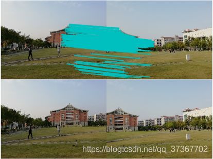
左边图与中间图落差较大些导致拼接痕迹比右边的明显。

3.2 室外 （景观落差大）

树木参差不齐，光线较暗，建筑较为相似，角度较高

落差大的图片失真率较高，拼接效果也比落差小的差，扭曲程度较大。

3.3  室内

原图：

sift特征匹配

图像拼接结果，黑板部分拼接效果不好，人多的地方拼接效果也不是好，由于sift特征匹配无法对边缘光滑的目标准确提取特征点而导致的。