Effective Approaches to Attention-based Neural Machine Translation_2015_Luong 【NMT】【Attention】
文章目录
- 提出背景
- 神经机器翻译NMT
- 模型
- Global Attention
- Local attention
- Input-feeding
论文链接:Effective Approaches to Attention-based Neural Machine Translation
By Luong et al. 2015
任务对齐(alignments between different modalities):对齐是指比如在翻译任务中,翻译每个词的时候,要找多需要重点关注的原句中的词,也就是将原文中的词和目标文中的词对应起来。
对齐权值(alignment weights):在翻译每个词的时候,需要关注那些encoder状态,关注的强度是多少,有一种打分机制,以前一刻的decoder状态和其中一个encoder状态为参数,输出得分 s c o r e ( h t , h ^ s ) score(h_t,\hat{h}_{s}) score(ht,h^s),然后用softmax归一化分值转换为概率,这个概率就是对齐权值。
Soft Attention: 软对齐,就是说encoder中每个词的隐藏层输出 h ^ s \hat{h}_{s} h^s都参与了权重的计算,这种方法方便反向传播。
Hard Attention: 就是会依赖encoder隐藏层的概率 S i S_i Si 选择部分进行计算,而不是整个encoder隐藏层。但是这种不放不可微想要实现梯度的反向传播,需要采用蒙特卡洛采样的方法估计模块的梯度。
提出背景
最新论文提出开始把注意力机制应用于neural machine translation (NMT),将注意力有选择地放在部分source sentence上,本文继续探索更好的将注意力机制应用在NMT。
提出两个模型,一个是Global Attention,将注意力放在全部的source sentence上,另一个是Local Attention,每一个时刻下将注意力放在部分source sentence上。Local Attention是融合了soft attention和hard attention,计算成本更小,而且可微(hard attention不可微),更容易实现和训练。
在对英语和德语互译上的实验中,local attention的BLEU值达到25.9,提高了1.0个点,global attention的BLEU值提升了5.0个点,优于当前使用dropout等技术的效果。
神经机器翻译NMT
nmt是一个神经网络,计算将原句 x 1 , x 2 , . . . x n x_1,x_2,...x_n x1,x2,...xn翻译成目标句 y 1 , y 2 , . . . y m y_1,y_2,...y_m y1,y2,...ym的条件概率: p ( y ∣ x ) p(y|x) p(y∣x)。
nmt的基本形式包括(1)encoder:计算source sentence的表示形式。(2)decoder:一次生成一个目标word,常用RNN结构实现。
已有的结构:
- CNN-RNN
- LSTM-LSTM
- GRU-GRU
模型
提出global和local两种模型,模型采用的是基于attention的stakcking LSTM architacture。
模型的共同点是decoding阶段每一次step t都将LSTM堆顶层作为 h t h_t ht的输入。目标是获得上下文向量 c t c_t ct,这个向量捕获原句中的信息来帮助预测当前的目标单词 y t y_t yt。
模型的不同点在于上下文向量 c t c_t ct是如何获取的。
给定目标隐藏层状态 h t h_t ht和上下文向量 c t c_t ct,使用一个连接层将这两个向量的信息结合,生成一个注意力层attentional hidden state:
h ^ t = tanh ( W c [ c t ; h t ] ) \hat{h}_{t}=\tanh(W_c[c_t;h_t]) h^t=tanh(Wc[ct;ht])
然后注意力向量作为softmax层的输入生成 y 的预测分布:
p ( y t ∣ y < t , x ) = s o f t m a x ( W s h ^ t ) p(y_t|y_{
下面是两个模型上下文向量计算思路的相似过程:
Global Attention
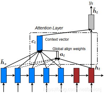
可变长对齐向量
可变长 理解为源句的长度不同,批量输入句子,不同的句子有不同维度的对齐向量 a t a_t at,或者句子不足最长的句子长度时,对应的单词的位置补0,将 a t a_t at理解为可变长的。
a t ( s ) = a l i g n ( h t , h ‾ s ) = exp ( s c o r e ( h t , h ‾ s ) ) ∑ s ′ exp ( s c o r e ( h t ) , h ‾ s ′ ) \begin{aligned} a_t(s)&=align(h_t,\overline{h}_s)\\ &=\frac{\exp(score(h_t,\overline{h}_s))}{\sum_{s^{'}}\exp(score(h_t),\overline{h}_s^{'})} \end{aligned} at(s)=align(ht,hs)=∑s′exp(score(ht),hs′)exp(score(ht,hs))
在step t 时刻,定义一个基于当前目标隐藏状态 h t h_t ht 和 源句每个隐藏状态 h ‾ s \overline{h}_{s} hs的对齐概率。
打分函数:
s c o r e ( h t , h ‾ s ) { h t T h ‾ s dot h t T W a h ‾ s general v a T tanh ( W a [ h t ; h ‾ s ] ) concat score(h_t,\overline{h}_s)\begin{cases} h_t^\mathsf{T}\overline{h}_s &\textit{dot}\\ h_t^\mathsf{T}W_a\overline{h}_s&\textit{general}\\ v_a\mathsf{T}\tanh(W_a[h_t;\overline{h}_s]) &\textit{concat} \end{cases} score(ht,hs)⎩⎪⎨⎪⎧htThshtTWahsvaTtanh(Wa[ht;hs])dotgeneralconcat
对源句每一个单词计算一个权重,对当前目标隐藏状态 h t h_t ht和每一个源句隐藏状态 h ‾ s \overline{h}_s hs,共提出并定义了三个content-based function打分函数,分别是dot,general和concat。
此外,还曾提出一个location-based function来计算对齐概率:
a t = s o f t m a x ( W a h t ) a_t=softmax(W_ah_t) at=softmax(Waht)
上下文向量:
c t = ∑ s a t ( s ) h ‾ s c_t=\sum_{s}a_t(s)\overline{h}_s ct=s∑at(s)hs
和Bahdanau et al.提出的soft attention机制(灵感来源)相比,更加简单,泛化能力更好之处在于:
- 本文使用encoder和decoder的最顶层隐藏层状态。原文使用双向编码器中的前向和后向源隐藏状态的串联以及非堆叠单向解码器中的目标隐藏状态。
- 本文计算思路更简单。本文计算路径: h t → a t → c t → h ~ t h_t \rightarrow a_t \rightarrow c_t \rightarrow \widetilde{h}_t ht→at→ct→h t,原文的计算思路是: h t − 1 → a t → c t → h t h_{t-1} \rightarrow a_t \rightarrow c_t \rightarrow h_t ht−1→at→ct→ht,从前一个隐藏层状态开始。
- 原文只是使用了一种对齐函数,即
concat product,而本文提出三种打分函数以供选择,结果显示第二种效果最好。
Local attention
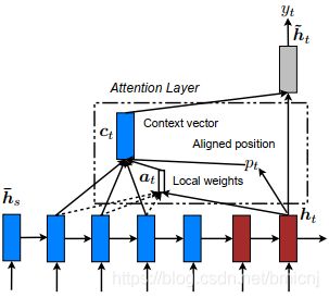
Global attention需要计算源句中的所有单词,计算代价高,当训练起来长文本,比如paragraph,document的时候,就不太适合。
Local attention有选择地将注意力放在一个小窗口中的文本内容,并且是可微的,避免了在同一时刻消耗过多的计算量,更容易训练。
为什么是可微的??理解不了!
在时刻 t t t 模型首先生成一个对齐位置 p t p_t pt,局部对齐向量 a t ( s ) a_t(s) at(s)和global attention的计算方式类似,源句隐藏状态窗口 [ p t − D , p t + D ] [p_t-D,p_t+D] [pt−D,pt+D] 的加权平均获得上下文向量 c t c_t ct,D是通过经验选择的。下面定义几个变量:
Monotonic alignment(local-m) 单调对齐:和soft attention一样。
a t ( s ) = a l i g n ( h t , h ‾ s ) = exp ( s c o r e ( h t , h ‾ s ) ) ∑ s ′ exp ( s c o r e ( h t ) , h ‾ s ′ ) \begin{aligned} a_t(s)&=align(h_t,\overline{h}_s)\\ &=\frac{\exp(score(h_t,\overline{h}_s))}{\sum_{s^{'}}\exp(score(h_t),\overline{h}_s^{'})} \end{aligned} at(s)=align(ht,hs)=∑s′exp(score(ht),hs′)exp(score(ht,hs))
将时刻 t 的对齐位置直接定义为 p t = t p_t=t pt=t。
Predictive alignment (local-p)预测对齐:
p t = S ⋅ s i g m o i d ( v p T tanh ( W p h t ) ) p_t=S\cdot{sigmoid(v_p^\mathsf{T}\tanh(W_ph_t))} pt=S⋅sigmoid(vpTtanh(Wpht))
将时刻 t 的对齐位置定义为一个预测出来的位置,S是源句的长度, W p , v p W_p,v_p Wp,vp是需要学习的参数,那么对齐中心位置的范围就是 p ∈ [ 0 , S ] p\in{[0,S]} p∈[0,S]。将 p t p_t pt作为均值 定义高斯函数来修正对齐函数 a t a_t at:
a t ( s ) = a l i g n ( h t , h ‾ s ) exp ( − ( s − p t ) 2 σ 2 ) a_t(s)=align(h_t,\overline{h}_s)\exp(-\frac{(s-p_t)}{2\sigma^2}) at(s)=align(ht,hs)exp(−2σ2(s−pt))
σ = D 2 \sigma=\frac{D}{2} σ=2D是经验值, p t p_t pt是一个表示位置的实数, s s s是以 p t p_t pt为中心的窗口中的一个整数。
Input-feeding
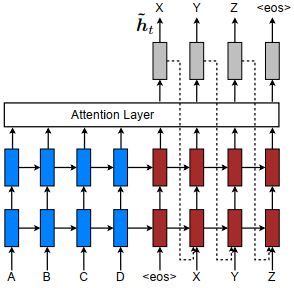
为了达到一种覆盖的效果,将当前的注意力隐藏状态也作为下一时刻的输入,达到两种目的:1.使模型完全了解以前的对齐状态。2.在横向和纵向上都建立了很深的神经网络。
global模型是在Bahdanau et al.(首次使用attention机制到机器翻译)的修改,创新点在于改变了对齐向量计算的思路,并且提出了不同的打分函数,经过不同的实验尝试,发现最好的method。
local模型是从图像生成领域Gregor et al.(2015)模型中将注意力放在a patch of image 受启发想到的思路,为了梯度可微,将软硬注意力机制混合。so,任务是不同的,思路是相通的…
参考:
https://zhuanlan.zhihu.com/p/52106264
http://flyrie.top/2018/12/25/Attention_Effective_Approaches_to_Attention-based_Neural_Machine_Translation/