PaddlePaddle学习课程——课节1：Python数据分析处理——Python数据分析入门

PaddlePaddle学习课程

课节1：Python数据分析处理

Python数据分析入门

波士顿房价的预测（数据分析和建模的初步知识）（附带相应知识的链接）

一、基础库介绍

1.Seaborn:

Seaborn是基于matplotlib的Python可视化库。 它提供了一个高级界面来绘制有吸引力的统计图形。Seaborn其实是在matplotlib的基础上进行了更高级的API封装，从而使得作图更加容易，不需要经过大量的调整就能使你的图变得精致。但应强调的是，应该把Seaborn视为matplotlib的补充，而不是替代物。

作者：W_hy
链接：https://www.jianshu.com/p/844f66d00ac1
来源：简书

2.XGBoost:

XGBoost可以成为机器学习的大杀器，广泛用于数据科学竞赛和工业界，是因为它有许多优点：

（1.使用许多策略去防止过拟合，如：正则化项、Shrinkage and Column Subsampling等。

（2. 目标函数优化利用了损失函数关于待求函数的二阶导数

（3.支持并行化，这是XGBoost的闪光点，虽然树与树之间是串行关系，但是同层级节点可并行。具体的对于某个节点，节点内选择最佳分裂点，候选分裂点计算增益用多线程并行。训练速度快。

（4.添加了对稀疏数据的处理。

（5.交叉验证，early stop，当预测结果已经很好的时候可以提前停止建树，加快训练速度。

（6.支持设置样本权重，该权重体现在一阶导数g和二阶导数h，通过调整权重可以去更加关注一些样本

原文链接：http://blog.itpub.net/31542119/viewspace-2199549/

3.Sklearn:

官方文档地址：https://scikit-learn.org/stable/
参考文档：https://www.cnblogs.com/wj-1314/p/10179741.html

5.Matplotlib

Matplotlib 是基于 NumPy 数组构建的多平台数据可视化库。它是John Hunter 在2002年构想的，原本的设计是给 IPython 打补丁，让命令行中也可以有交互式的 MATLAB 风格的画图工具。

在近些年，已经出现了更新更好的工具最终替代了 Matplotlib（比如 R 语言中的ggplot和ggvis）， 但 Matplotlib 依旧是一个经过良好测试的、跨平台的图形引擎。
http://www.sohu.com/a/318173714_464033

二、代码详情

安装或导入必要的package

!pip install seaborn
!pip install xgboost
!pip install sklearn

import pandas as pd
import numpy as np
import seaborn as sns
import matplotlib as mpl

import matplotlib.pyplot as plt
from IPython.display import display
plt.style.use("fivethirtyeight")
sns.set_style({'font.sans-serif':['simhei','Arial']})
%matplotlib inline

#导入数据
housing = pd.read_csv('E:\\Anaconda\\work\\Paddlepaddle\\learning\\housingPrices_train.csv')

display(housing.head(n=5))#显示数据前5个

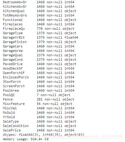
housing.info()#信息统计

housing.describe()#信息描述

可视化处理

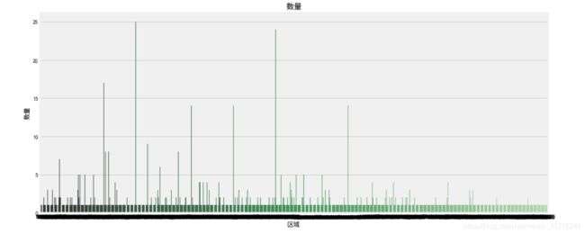
# 对区域分组对比每平米房价
housing_count = housing.groupby('LotArea')['SalePrice'].count().sort_values(ascending=False).to_frame().reset_index()


f, [ax2,ax3] = plt.subplots(2,1,figsize=(15,15))#几个子图，


sns.barplot(x='LotArea', y='SalePrice', palette="Greens_d", data=housing_count, ax=ax2)#条形图
ax2.set_title('数量',fontsize=15)
ax2.set_xlabel('区域')
ax2.set_ylabel('数量')

sns.boxplot(x='LotArea', y='SalePrice', data=housing, ax=ax3)
ax3.set_title('总价',fontsize=15)
ax3.set_xlabel('区域')
ax3.set_ylabel('房屋总价')

plt.show()

groupby:进行分组，并且进行组内运算
分组统计GroupBy技术详解：https://blog.csdn.net/Asher117/article/details/85614034
关于男女分组的具体应用：https://blog.csdn.net/shujuelin/article/details/79635848

f, [ax1,ax2] = plt.subplots(1, 2, figsize=(15, 5))#figsize为设定的尺寸
# 建房时间的分布情况
sns.distplot(housing['YearBuilt'], bins=20, ax=ax1, color='r')#displot()集合了matplotlib的hist()与核函数估计kdeplot的功能，增加了rugplot分布观测条显示与利用scipy库fit拟合参数分布的新颖用途。
sns.kdeplot(housing['YearBuilt'], shade=True, ax=ax1)#核密度估计图
# 建房时间和出售价格的关系
sns.regplot(x='YearBuilt', y='SalePrice', data=housing, ax=ax2)
plt.show()

subplots详解：https://blog.csdn.net/htuhxf/article/details/82986440

具体的几种图像在上方seaborn连接中。

#缺失值查找
misn = len(housing.loc[(housing['Fence'].isnull()), 'Fence'])
print('Fence缺失值数量为：'+ str(misn))

loc：通过行标签索引数据

iloc：通过行号索引行数据

ix：通过行标签或行号索引数据（基于loc和iloc的混合）

特征工程

在机器学习的具体实践任务中，选择一组具有代表性的特征用于构建模型是非常重要的问题。特征选择通常选择与类别相关性强、且特征彼此间相关性弱的特征子集，具体特征选择算法通过定义合适的子集评价函数来体现。在现实世界中，数据通常是复杂冗余，富有变化的，有必要从原始数据发现有用的特性。人工选取出来的特征依赖人力和专业知识，不利于推广。于是我们需要通过机器来学习和抽取特征，促进特征工程的工作更加快速、有效。特征选择的目标是寻找最优特征子集

对波士顿房价数据做特征工程

数据预处理要点： 1.使用log（x+1）来转换偏斜的数字特征 -，这将使我们的数据更加正常 2.为分类要素创建虚拟变量 3.将数字缺失值（NaN）替换为各自列的平均值

import pandas as pd
import numpy as np
from scipy.stats import skew
import xgboost as xgb
from sklearn.model_selection  import KFold
from sklearn.ensemble import ExtraTreesRegressor
from sklearn.ensemble import RandomForestRegressor
from sklearn.metrics import mean_squared_error
from sklearn.linear_model import Ridge, RidgeCV, ElasticNet, LassoCV, Lasso
from math import sqrt

参数设置

TARGET = 'SalePrice'
NFOLDS = 5#K-Fold 交叉验证 (Cross-Validation)中的组数
SEED = 0
NROWS = None
SUBMISSION_FILE = 'E:\\Anaconda\\work\\Paddlepaddle\\learning\\sample_submission.csv'
  
## Load the data ##
train = pd.read_csv("E:\\Anaconda\\work\\Paddlepaddle\\learning\\housingPrices_train.csv")
test = pd.read_csv("E:\\Anaconda\\work\\Paddlepaddle\\learning\\housingPrices_test.csv")

ntrain = train.shape[0]#1460
ntest = test.shape[0]#1459

y_train = np.log(train[TARGET]+1)

train.drop([TARGET],axis = 1, inplace = True)#删除指定范围

all_data = pd.concat((train.loc[:,'MSSubClass':'SaleCondition'],
                       test.loc[:,'MSSubClass':'SaleCondition']))#数据合并与重塑

pd.concat详解：https://blog.csdn.net/mr_hhh/article/details/79488445

#log transform skewed numeric features
numer_feats = all_data.dtypes[all_data.dtypes != "object"].index

保留非"object"元素

skewed_feats1 = train[numer_feats].apply(lambda x: skew(x.dropna()))#运用偏度以及过滤缺失值
skewed_feats2 = skewed_feats1[skewed_feats1 > 0.75]#利用偏度缩小范围,设为0.75原因是因为skew 太高的情况下，特征值会有较为严重的 shake up，特征的变化对于 模型的影响很大。这里选的是>0.75，选的大的，可以发现偏得很严重。
skewed_feats3 = skewed_feats2.index#保留skewed_feats2的索引

dropna详解：https://blog.csdn.net/weixin_40283816/article/details/84304055

all_data[skewed_feats3] = np.log1p(all_data[skewed_feats3])#平滑化数据，使其符合正态分布

all_data = pd.get_dummies(all_data)#哑变量编码,类似于独热编码

dummies详解：https://www.jianshu.com/p/5f8782bf15b1

#filling NA's with the mean of the column:
all_data =all_data.fillna(all_data.mean())#将空缺的位置填充平均值

#creating matrices for sklearn:
x_train = np.array(all_data[:train.shape[0]])
x_test = np.array(all_data[train.shape[0]:])

kf = KFold(NFOLDS,shuffle=True,random_state=SEED)

关于kfold的一些其他解释及应用：
https://www.jianshu.com/p/284581d9b189

https://blog.csdn.net/GitzLiu/article/details/82670315

https://blog.csdn.net/accumulate_zhang/article/details/78490394

class SklearnWrapper(object):
    def __init__(self,clf,seed=0,params=None):
        params['random_state'] = seed
        self.clf = clf(**params)
        
    def train(self,x_train,y_train):
        self.clf.fit(x_train,y_train)#训练方法，可设置值。表示用数据X来训练某种模型。 函数返回值一般为调用fit方法的对象本身。fit(X,y=None)为无监督学习算法，fit(X,Y)为监督学习算法
        
    def predict(self,x):
        return self.clf.predict(x)

class XgbWrapper(object):
    def __init__(self,seed=0,params=None):
        self.param = params
        self.param['seed'] = seed
        self.nrounds = params.pop('nrounds',250)
        
    def train(self,x_train,y_train):
        dtrain = xgb.DMatrix(x_train,label = y_train)
        self.gbdt = xgb.train(self.param,dtrain,self.nrounds)
        
    def predict(self,x):
        return self.gbdt.predict(xgb.DMatrix(x))

#clf是选择的分类模型，x_train是所有训练集，y_train是所有训练集样本的类别标签，x_test是给定的所有测试集
def get_oof(clf):
    oof_train = np.zeros((ntrain,))#全0array
    oof_test = np.zeros((ntest,))#全0array
    oof_test_skf = np.empty((10,ntest))#一个用随机值填充的矩阵，用来存放10次交叉后的预测结果
    #10次交叉，10次循环
    #kf实际上是一个迭代器，是从样本中分成了10组训练集和测试集的索引号
    for i,(train_index, test_index) in enumerate(kf.split(x_train)):
        #train
        x_tr = x_train[train_index]#当前循环，当前实验的训练数据
        y_tr = y_train[train_index]#当前循环的训练数据标签
        #test
        x_te = x_train[test_index]#当前循环的测试数据
        
        clf.train(x_tr,y_tr)#用模型去拟合数据，也就是训练预测模型
        
        oof_train[test_index] = clf.predict(x_te)#把测试数据的预测标签按照对应索引，放到oof_train对应索引处
        oof_test_skf[i, :] = clf.predict(x_test)#用当前的模型，预测所有测试数据的标签，并放到oof_test_skf的一行中
        
    #10次实验做完，把10次得到的结果求平均
    oof_test[:] = oof_test_skf.mean(axis=0)
    return oof_train.reshape(-1,1),oof_test.reshape(-1,1)

#进行查看
for i,(train_index, test_index) in enumerate(kf.split(x_train)):
    print (i,train_index,test_index)

可发现已经分成了10组

et_params = {
    'n_jobs': 16,
    'n_estimators': 100,
    'max_features': 0.5,
    'max_depth': 12,
    'min_samples_leaf': 2,
}
 
rf_params = {
    'n_jobs': 16,
    'n_estimators': 100,
    'max_features': 0.2,
    'max_depth': 12,
    'min_samples_leaf': 2,
}
 
xgb_params = {
    'seed': 0,
    'colsample_bytree': 0.7,
    'silent': 1,
    'subsample': 0.7,
    'learning_rate': 0.075,
    'objective': 'reg:linear',
    'max_depth': 4,
    'num_parallel_tree': 1,
    'min_child_weight': 1,
    'eval_metric': 'rmse',
    'nrounds': 500
}
 

rd_params={
    'alpha': 10
}
 
ls_params={
    'alpha': 0.005
}

各种模型的参数设置

xg = XgbWrapper(seed = SEED,params=xgb_params)
et = SklearnWrapper(clf = ExtraTreesRegressor,seed = SEED, params = et_params)#极端随机森林
rf = SklearnWrapper(clf = RandomForestRegressor, seed = SEED, params = rf_params)#随机森林
rd = SklearnWrapper(clf = Ridge, seed = SEED, params = rd_params)#岭回归
ls = SklearnWrapper(clf = Lasso, seed = SEED, params = ls_params)#LASSO回归

xg_oof_train, xg_oof_test = get_oof(xg)
et_oof_train, et_oof_test = get_oof(et)
rf_oof_train, rf_oof_test = get_oof(rf)
rd_oof_train, rd_oof_test = get_oof(rd)
ls_oof_train, ls_oof_test = get_oof(ls)

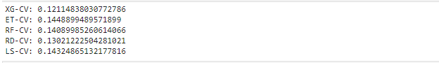
print("XG-CV: {}".format(sqrt(mean_squared_error(y_train, xg_oof_train))))
print("ET-CV: {}".format(sqrt(mean_squared_error(y_train, et_oof_train))))
print("RF-CV: {}".format(sqrt(mean_squared_error(y_train, rf_oof_train))))
print("RD-CV: {}".format(sqrt(mean_squared_error(y_train, rd_oof_train))))
print("LS-CV: {}".format(sqrt(mean_squared_error(y_train, ls_oof_train))))

x_train = np.concatenate((xg_oof_train, et_oof_train, rf_oof_train, rd_oof_train, ls_oof_train), axis=1)
x_test = np.concatenate((xg_oof_test, et_oof_test, rf_oof_test, rd_oof_test, ls_oof_test), axis=1)

print("{},{}".format(x_train.shape, x_test.shape))

dtrain = xgb.DMatrix(x_train, label=y_train)
dtest = xgb.DMatrix(x_test)

xgb_params = {
    'seed': 0,
    'colsample_bytree': 0.8,
    'silent': 1,
    'subsample': 0.6,
    'learning_rate': 0.01,
    'objective': 'reg:linear',
    'max_depth': 1,
    'num_parallel_tree': 1,
    'min_child_weight': 1,
    'eval_metric': 'rmse',
}

res = xgb.cv(xgb_params, dtrain, num_boost_round=1000, nfold=4, seed=SEED, stratified=False,
             early_stopping_rounds=25, verbose_eval=10, show_stdv=True)

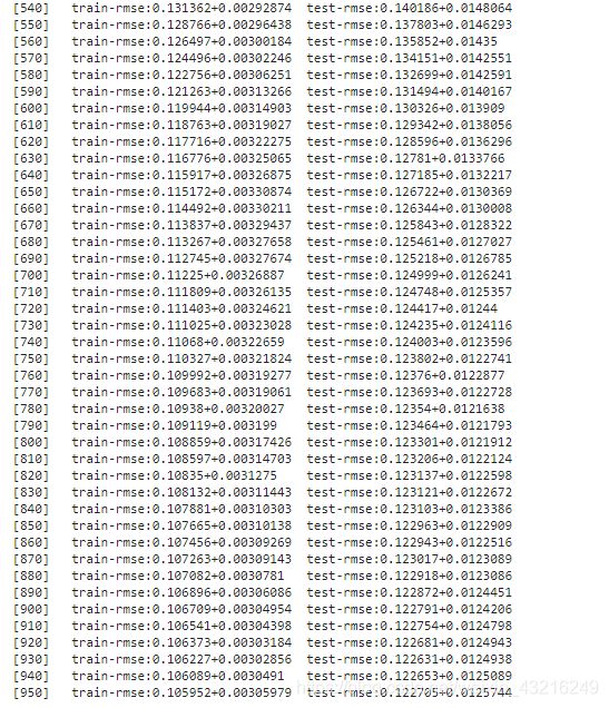
best_nrounds = res.shape[0] - 1
cv_mean = res.iloc[-1, 0]
cv_std = res.iloc[-1, 1]

print('Ensemble-CV: {0}+{1}'.format(cv_mean, cv_std))

gbdt = xgb.train(xgb_params, dtrain, best_nrounds)

!cat /dev/null > sample_submission.csv#创建相应文件

submission = pd.read_csv(SUBMISSION_FILE,engine = 'python',encoding = 'utf-8')
submission.iloc[:,0] = gbdt.predict(dtest)
saleprice = np.exp(submission['SalePrice'])-1
submission['SalePrice'] = saleprice
submission.to_csv('xgstacker_starter.sub.csv', index=None)

写入结果

三、遇见的问题

1、TypeError: ‘KFold’ object is not iterable：

主要是参数NFOLDS的设置，必须一一对应，另外在进行迭代的时候，如下：

for i, (train_index, test_index) in enumerate(kf):
        x_tr = x_train[train_index]
        y_tr = y_train[train_index]
        x_te = x_train[test_index]

如是使用enumerate(kf)，则是可能出现问题的，所以在查阅之后，我改成了以下代码：

for i,(train_index, test_index) in enumerate(kf.split(x_train)):
        #train
        x_tr = x_train[train_index]#当前循环，当前实验的训练数据
        y_tr = y_train[train_index]#当前循环的训练数据标签
        #test
        x_te = x_train[test_index]#当前循环的测试数据

问题解决

2. No columns to parse from file

解决方法：在本地用Excel创建一个csv文件，注意要用UTF-8格式保存。另外,文件开头需要写入”SalePrice"，在后面会用到。

问题解决

应用的数据集，等下会一起发布，有问题可以私戳。