吴恩达机器学习作业（二）实现：logistic回归

对于这一类分类问题：

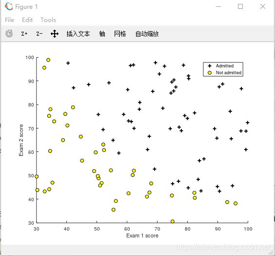
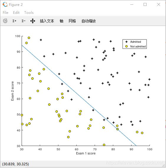
拿到数据先将它绘制出来，看数据在图片的分布，如果明显是两极化的，就用普通的逻辑回归，
比如下图：

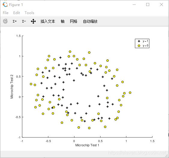
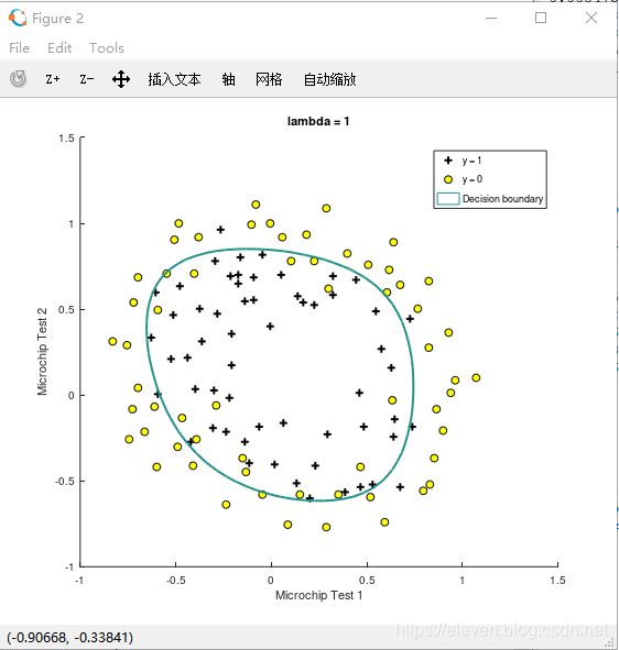
如果数据的分布比较特别，就加入正则化，所谓正则化就是加入惩罚项，使得结果不容易过度拟合，所以两者只有代价函数不一样
比如下图：

当然还有更高级的回归算法，这是比较常用且简单的算法

ex2.m

所有编写的函数都在这里面调用

%% Machine Learning Online Class - Exercise 2: Logistic Regression
%
%  Instructions
%  ------------
% 
%  This file contains code that helps you get started on the logistic
%  regression exercise. You will need to complete the following functions 
%  in this exericse:
%
%     sigmoid.m
%     costFunction.m
%     predict.m
%     costFunctionReg.m
%
%  For this exercise, you will not need to change any code in this file,
%  or any other files other than those mentioned above.
%

%% Initialization
clear ; close all; clc

%% Load Data
%  The first two columns contains the exam scores and the third column
%  contains the label.

data = load('ex2data1.txt');
X = data(:, [1, 2]); y = data(:, 3);

%% ==================== Part 1: Plotting ====================
%  We start the exercise by first plotting the data to understand the 
%  the problem we are working with.

fprintf(['Plotting data with + indicating (y = 1) examples and o ' ...
         'indicating (y = 0) examples.\n']);

plotData(X, y);

% Put some labels 
hold on;
% Labels and Legend
xlabel('Exam 1 score')
ylabel('Exam 2 score')

% Specified in plot order
legend('Admitted', 'Not admitted')
hold off;

fprintf('\nProgram paused. Press enter to continue.\n');
pause;


%% ============ Part 2: Compute Cost and Gradient ============
%  In this part of the exercise, you will implement the cost and gradient
%  for logistic regression. You neeed to complete the code in 
%  costFunction.m

%  Setup the data matrix appropriately, and add ones for the intercept term
[m, n] = size(X);

% Add intercept term to x and X_test
X = [ones(m, 1) X];

% Initialize fitting parameters
initial_theta = zeros(n + 1, 1);

% Compute and display initial cost and gradient
[cost, grad] = costFunction(initial_theta, X, y);

fprintf('Cost at initial theta (zeros): %f\n', cost);
fprintf('Expected cost (approx): 0.693\n');
fprintf('Gradient at initial theta (zeros): \n');
fprintf(' %f \n', grad);
fprintf('Expected gradients (approx):\n -0.1000\n -12.0092\n -11.2628\n');

% Compute and display cost and gradient with non-zero theta
test_theta = [-24; 0.2; 0.2];
[cost, grad] = costFunction(test_theta, X, y);

fprintf('\nCost at test theta: %f\n', cost);
fprintf('Expected cost (approx): 0.218\n');
fprintf('Gradient at test theta: \n');
fprintf(' %f \n', grad);
fprintf('Expected gradients (approx):\n 0.043\n 2.566\n 2.647\n');

fprintf('\nProgram paused. Press enter to continue.\n');
pause;


%% ============= Part 3: Optimizing using fminunc  =============
%  In this exercise, you will use a built-in function (fminunc) to find the
%  optimal parameters theta.

%  Set options for fminunc
options = optimset('GradObj', 'on', 'MaxIter', 400);

%  Run fminunc to obtain the optimal theta
%  This function will return theta and the cost 
[theta, cost] = ...
	fminunc(@(t)(costFunction(t, X, y)), initial_theta, options);

% Print theta to screen
fprintf('Cost at theta found by fminunc: %f\n', cost);
fprintf('Expected cost (approx): 0.203\n');
fprintf('theta: \n');
fprintf(' %f \n', theta);
fprintf('Expected theta (approx):\n');
fprintf(' -25.161\n 0.206\n 0.201\n');

% Plot Boundary
plotDecisionBoundary(theta, X, y);%已给函数

% Put some labels 
hold on;
% Labels and Legend
xlabel('Exam 1 score')
ylabel('Exam 2 score')

% Specified in plot order
legend('Admitted', 'Not admitted')
hold off;

fprintf('\nProgram paused. Press enter to continue.\n');
pause;

%% ============== Part 4: Predict and Accuracies ==============
%  After learning the parameters, you'll like to use it to predict the outcomes
%  on unseen data. In this part, you will use the logistic regression model
%  to predict the probability that a student with score 45 on exam 1 and 
%  score 85 on exam 2 will be admitted.
%
%  Furthermore, you will compute the training and test set accuracies of 
%  our model.
%
%  Your task is to complete the code in predict.m

%  Predict probability for a student with score 45 on exam 1 
%  and score 85 on exam 2 

prob = sigmoid([1 45 85] * theta);
fprintf(['For a student with scores 45 and 85, we predict an admission ' ...
         'probability of %f\n'], prob);
fprintf('Expected value: 0.775 +/- 0.002\n\n');

% Compute accuracy on our training set
p = predict(theta, X);

fprintf('Train Accuracy: %f\n', mean(double(p == y)) * 100);
fprintf('Expected accuracy (approx): 89.0\n');
fprintf('\n');

1.1 plotData.m

这个函数是用来绘制数据的

function plotData(X, y)
%PLOTDATA Plots the data points X and y into a new figure 
%   PLOTDATA(x,y) plots the data points with + for the positive examples
%   and o for the negative examples. X is assumed to be a Mx2 matrix.

% Create New Figure
figure; hold on;

% ====================== YOUR CODE HERE ======================
% Instructions: Plot the positive and negative examples on a
%               2D plot, using the option 'k+' for the positive
%               examples and 'ko' for the negative examples.
%

% Find Indices of Positive and Negative Examples

pos = find(y==1); 
neg = find(y == 0);
% Plot Examples
%设置录取的是+，未录取的是o,并设置相关属性
plot(X(pos, 1), X(pos, 2), 'k+','LineWidth', 2, ...'MarkerSize', 7);
plot(X(neg, 1), X(neg, 2), 'ko', 'MarkerFaceColor', 'y', ...'MarkerSize', 7);

% =========================================================================

hold off;

end

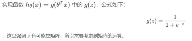
1.2.1 sigmoid.m

function g = sigmoid(z)
%SIGMOID Compute sigmoid function
%   g = SIGMOID(z) computes the sigmoid of z.

% You need to return the following variables correctly 
g = zeros(size(z));

% ====================== YOUR CODE HERE ======================
% Instructions: Compute the sigmoid of each value of z (z can be a matrix,
%               vector or scalar).

g = 1 ./ (ones(size(z)) + e .^ (-z));

% =============================================================

end

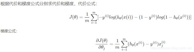
1.2.2 costFunction.m

function [J, grad] = costFunction(theta, X, y)
%COSTFUNCTION Compute cost and gradient for logistic regression
%   J = COSTFUNCTION(theta, X, y) computes the cost of using theta as the
%   parameter for logistic regression and the gradient of the cost
%   w.r.t. to the parameters.

% Initialize some useful values
m = length(y); % number of training examples

% You need to return the following variables correctly 
J = 0;
grad = zeros(size(theta));

% ====================== YOUR CODE HERE ======================
% Instructions: Compute the cost of a particular choice of theta.
%               You should set J to the cost.
%               Compute the partial derivatives and set grad to the partial
%               derivatives of the cost w.r.t. each parameter in theta
%
% Note: grad should have the same dimensions as theta
%

h_theta = sigmoid(X * theta); % X: m * n theta: n * 1 h_theta: m * 1

J = (-y' * log(h_theta) - (1 - y)' * log(1 - h_theta)) / m; % y: m * 1
grad = X' * (h_theta - y) / m;

% =============================================================

end

1.2.4 predict.m

预测函数，返回判断结果为 0 or 1。

function p = predict(theta, X)
%PREDICT Predict whether the label is 0 or 1 using learned logistic 
%regression parameters theta
%   p = PREDICT(theta, X) computes the predictions for X using a 
%   threshold at 0.5 (i.e., if sigmoid(theta'*x) >= 0.5, predict 1)

m = size(X, 1); % Number of training examples

% You need to return the following variables correctly
p = zeros(m, 1);

% ====================== YOUR CODE HERE ======================
% Instructions: Complete the following code to make predictions using
%               your learned logistic regression parameters. 
%               You should set p to a vector of 0's and 1's
%

p = sigmoid(X * theta) > 0.5;      % X: m * n     theta: n * 1

% =========================================================================


end

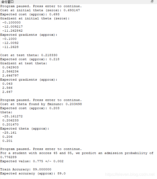
结果：

这是绘制出来的图片

正则化

ex2_reg.m

%% Machine Learning Online Class - Exercise 2: Logistic Regression
%
%  Instructions
%  ------------
%
%  This file contains code that helps you get started on the second part
%  of the exercise which covers regularization with logistic regression.
%
%  You will need to complete the following functions in this exericse:
%
%     sigmoid.m
%     costFunction.m
%     predict.m
%     costFunctionReg.m
%
%  For this exercise, you will not need to change any code in this file,
%  or any other files other than those mentioned above.
%

%% Initialization
clear ; close all; clc

%% Load Data
%  The first two columns contains the X values and the third column
%  contains the label (y).

data = load('ex2data2.txt');
X = data(:, [1, 2]); y = data(:, 3);

plotData(X, y);

% Put some labels
hold on;

% Labels and Legend
xlabel('Microchip Test 1')
ylabel('Microchip Test 2')

% Specified in plot order
legend('y = 1', 'y = 0')
hold off;


%% =========== Part 1: Regularized Logistic Regression ============
%  In this part, you are given a dataset with data points that are not
%  linearly separable. However, you would still like to use logistic
%  regression to classify the data points.
%
%  To do so, you introduce more features to use -- in particular, you add
%  polynomial features to our data matrix (similar to polynomial
%  regression).
%

% Add Polynomial Features

% Note that mapFeature also adds a column of ones for us, so the intercept
% term is handled
X = mapFeature(X(:,1), X(:,2));

% Initialize fitting parameters
initial_theta = zeros(size(X, 2), 1);

% Set regularization parameter lambda to 1
lambda = 1;

% Compute and display initial cost and gradient for regularized logistic
% regression
[cost, grad] = costFunctionReg(initial_theta, X, y, lambda);

fprintf('Cost at initial theta (zeros): %f\n', cost);
fprintf('Expected cost (approx): 0.693\n');
fprintf('Gradient at initial theta (zeros) - first five values only:\n');
fprintf(' %f \n', grad(1:5));
fprintf('Expected gradients (approx) - first five values only:\n');
fprintf(' 0.0085\n 0.0188\n 0.0001\n 0.0503\n 0.0115\n');

fprintf('\nProgram paused. Press enter to continue.\n');
pause;

% Compute and display cost and gradient
% with all-ones theta and lambda = 10
test_theta = ones(size(X,2),1);
[cost, grad] = costFunctionReg(test_theta, X, y, 10);

fprintf('\nCost at test theta (with lambda = 10): %f\n', cost);
fprintf('Expected cost (approx): 3.16\n');
fprintf('Gradient at test theta - first five values only:\n');
fprintf(' %f \n', grad(1:5));
fprintf('Expected gradients (approx) - first five values only:\n');
fprintf(' 0.3460\n 0.1614\n 0.1948\n 0.2269\n 0.0922\n');

fprintf('\nProgram paused. Press enter to continue.\n');
pause;

%% ============= Part 2: Regularization and Accuracies =============
%  Optional Exercise:
%  In this part, you will get to try different values of lambda and
%  see how regularization affects the decision coundart
%
%  Try the following values of lambda (0, 1, 10, 100).
%
%  How does the decision boundary change when you vary lambda? How does
%  the training set accuracy vary?
%

% Initialize fitting parameters
initial_theta = zeros(size(X, 2), 1);

% Set regularization parameter lambda to 1 (you should vary this)
lambda = 1;

% Set Options
options = optimset('GradObj', 'on', 'MaxIter', 400);

% Optimize
[theta, J, exit_flag] = ...
	fminunc(@(t)(costFunctionReg(t, X, y, lambda)), initial_theta, options);

% Plot Boundary
plotDecisionBoundary(theta, X, y);
hold on;
title(sprintf('lambda = %g', lambda))

% Labels and Legend
xlabel('Microchip Test 1')
ylabel('Microchip Test 2')

legend('y = 1', 'y = 0', 'Decision boundary')
hold off;

% Compute accuracy on our training set
p = predict(theta, X);

fprintf('Train Accuracy: %f\n', mean(double(p == y)) * 100);
fprintf('Expected accuracy (with lambda = 1): 83.1 (approx)\n');

2.3 costFunctionReg.m

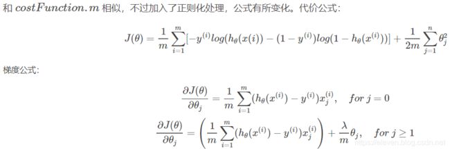
function [J, grad] = costFunctionReg(theta, X, y, lambda)
%COSTFUNCTIONREG Compute cost and gradient for logistic regression with regularization
%   J = COSTFUNCTIONREG(theta, X, y, lambda) computes the cost of using
%   theta as the parameter for regularized logistic regression and the
%   gradient of the cost w.r.t. to the parameters. 

% Initialize some useful values
m = length(y); % number of training examples

% You need to return the following variables correctly 
J = 0;
grad = zeros(size(theta));

% ====================== YOUR CODE HERE ======================
% Instructions: Compute the cost of a particular choice of theta.
%               You should set J to the cost.
%               Compute the partial derivatives and set grad to the partial
%               derivatives of the cost w.r.t. each parameter in theta

h_theta = sigmoid(X * theta); % X: m * n theta: n * 1 h_theta: m * 1

J = (-y' * log(h_theta) - (1 - y)' * log(1 - h_theta)) / m + ...
    lambda * (theta' * theta - (theta(1, 1))^2) / (2 * m); % y: m * 1
theta(1) = 0;
grad = (X' * (h_theta - y) + theta * lambda) / m;

% =============================================================

end

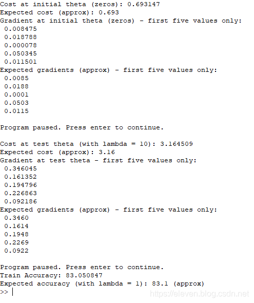
正则化的结果：

以及一些我看到的比较好 的用py实现的例子：

用python实现逻辑回归1
用python实现逻辑回归2