LCA: Loss Change Allocation for Neural Network Training (神经网络在训练过程中的损失变化分配)

Paper in here.   Code in here.   Uber Blog in here.   Video in here

Motivation

  The empirical tell us that loss will decrease when we training the neural network if we properly designed the network architecture and neural algorithm. In other words, the loss change index the convergence of the algorithm or learn efficient of the neural network or not. However, if we allocation the loss to every parameters of the neural network, the loss change of the parameters will be obtained. We will be find that which parameters will be decrease the totally loss to help neural convergence, and which increase the loss to hurt the SGD convergence to local minima point.

  经验告诉我们，随着网络的训练，损失是会下降的（假设所有设计都正确），损失函数的变化指示着算法的收敛性和网路的学习过程。然而，当我们把总体的损失函数分配到网络中的每一个参数上，来具体测量损失在每个参数上的变化程度，结果会怎样？这篇文章，就是基于这样的思路，对每层、没通道甚至没个神经元的损失变化情况进行了测量，该方法将得到那些有意思的结论呢？

Some Useful Conclusion of LCA

• We find that barely over 50% of parameters help during any given iteration.
  在任何迭代过程中，只有50%的参数对减少损失是有益的。
• Some entire layers hurt overall, moving on average against the training gradient, a phenomenon we hypothesize may be due to phase lag in an oscillatory training process.
  有些层整体对损失减少有害，并逆着梯度移动向一个平均点，作者将该现象解释为一种在震荡训练过程中的阶段滞后。
• Finally, increments in learning proceed in a synchronized manner across layers, often peaking on identical iterations.
  最后，学习的增量以同步的方式跨层进行，通常在相同的迭代中达到峰值。

What is the LCA?

  We propose a new window into training called Loss Change Allocation (LCA), in which credit for changes to the network loss is conservatively partitioned to the parameters. This measurement is accomplished by decomposing the components of an approximate path integral along the training trajectory using a Runge-Kutta integrator.
  In one word, it is a simple approach to inspecting training in progress by decomposing changes in the overall network loss into a per-parameter Loss Change Allocation or LCA.

  作者关于网络训练提出了一个新的视角，叫做损失变化分配（LCA）。在 LCA 中，网络损失变化的信誉（Credit）被适当地划分到其参数上。这种测量是通过使用 Runge-Kutta (RK4) 积分器 (用于非线性常微分方程的解的重要的一类隐式或显式迭代法) 沿训练轨迹分解近似路径积分的分量来完成的。
  总的来说，提出了一种检测 每个网络参数上 loss 变化的方法。

Methods

  This rich view shows which parameters are responsible for decreasing or increasing the loss during training, or which parameters “help” or “hurt” the network’s learning, respectively.
  该视角显示了在网络训练过程中,那些参数可以减少 (means help) 或增加 (means hurt) 损失，并给出了具体的量化方法（loss change on per parameters）。

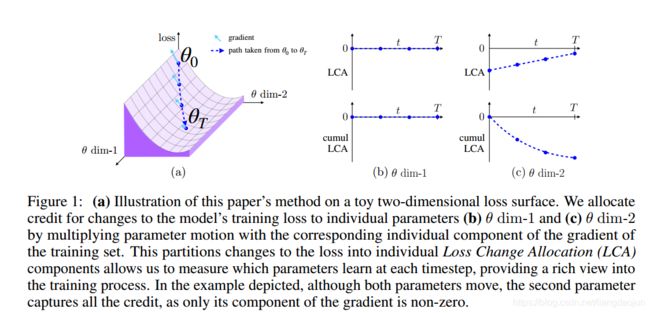
  Negative LCA and is “helping” or “learning”. Positive LCA is “hurting” the learning process, which may result from several causes: a noisy mini-batch with the gradient of that step going the wrong way, momentum, or a step size that is too large for a curvy or rugged loss landscape. If the parameter has a non-zero gradient but does not move, it does not affect the loss. Figure 1 depicts a toy example using two parameters.

  负的 LCA 是有帮助的，正的 LCA 是有害的，他可能是 mini-batch 的gradient走了错误的方向和大的崎岖的曲线而产生的。0 gradient 不产生移动。上图是一个两个参数的toy example.

  Consider a parameterized training scenario where a model starts at parameter value ${\theta }_0$ and ends at parameter value ${\theta }_T$ after training. The training process entails traversing some path P along the surface of a loss landscape from ${\theta }_0$ to ${\theta }_T$ . The loss change can derives from a straightforward application of the fundamental theorem of calculus to a path integral along the loss landscape:
  考虑网络参数在0时刻 ${\theta }_0$ 到T时刻 ${\theta }_T$ 沿着路径 P 变化, 对该路径进行积分可以得到：

where C is any path from ${\theta }_0$ to ${\theta }_T$ and <.,.> is the dot product. This equation states that the change in loss from θ0 to θT may be calculated by integrating the dot product of the loss gradient and parameter motion along a path from ${\theta }_0$ to ${\theta }_T$ . Because ${▽}_{\theta }L(\theta )$ is the gradient of a function and thus is a conservative field, any path from ${\theta }_0$ to ${\theta }_T$ may be used.
其中，C是${\theta }_0$ 到 ${\theta }_T$的任意的路径，<.,.>是点积（dot product）。该等是描述了${\theta }_0$ 到 ${\theta }_T$参数移动的情况。${▽}_{\theta }L(\theta )$ 是梯度函数，因为标量场的梯度是保守场，保守场的第二类曲线积分只与起点和终点有关，而与路径无关 （就像重力做功一样），保守场的第二个性质是旋度都是零，即无旋矢量场，这里只讨论第一个性质。

  We may approximate this path integral from ${\theta }_0$ to ${\theta }_T$ by using a series of first order Taylor approximations along the training path. If we index training steps by $t\in [0;1;\dots ;T]$, the first order approximation for the change in loss during one step of training is the following, rewritten as a sum of its individual components:
使用 ${\theta }_0$ 到 ${\theta }_T$ 的参数序列来近似路径积分，那么，（1）式中的 1 阶泰勒展开在各个分量和的形式就可以表示为：

where ${▽}_{\theta }L({\theta }_t)$ represents the gradient of the loss of the whole training set w.r.t. θ evaluated at ${\theta }_t$, $v(i)$ represents the $i$-th element of a vector $v$, and the parameter vector θ contains K elements. Note that while we evaluate model learning by tracking progress along the training set loss landscape $L(\theta )$.

${▽}_{\theta }L({\theta }_t)$是整个数据集在 ${\theta }_t$ 时的损失 ($t$-th epoch?)。上标 i 代表第 i 个分量。

  As shown in Equation 3, the difference in loss produced by one training iteration t may be decomposed into K individual Loss Change Allocation, or LCA, components, denoted $A_{t,i}$. These K components represent the LCA for a single iteration of training, and over the course of T iterations of training we will collect a large T × K matrix of $A_{t,i}$ values.

  每个参数由 K个分量，网络使用 SGD 或 Adam 训练 T 个时间步（epoch），将产生一个 T x K 个 $A_{t,i}$ 值。

Property of LCA

  This is in contrast to approaches that measure quantities like parameter motion or approximate elements of the Fisher information (FI) , which also produce per-parameter measurements but depend heavily on the parameterization chosen. For example, the FI metric is sensitive to scale (e.g. multiply one relu layer weights by 2 and next by 0.5: loss stays the same but FI of each layer changes and total FI changes).

  对比Fisher information (FI) 方法，其主要测量参数移动或者元素逼近，它严重依赖参数的选择，而且对 尺度 敏感。比如，在前层的Relu 乘以2，在后层乘以 0.5，得到的FI是一样的。

  We can improve on our LCA approximation from Equation 2 by replacing ${\nabla }_{\theta }L({\theta }_t)$ with $\frac{1}{6}({\nabla }_{\theta }L({\theta }_t)+4{\nabla }_{\theta }L(\frac{1}{2}{\theta }_t+\frac{1}{2}{\theta }_{t+1})+{\nabla }_{\theta }L({\theta }_{t+1}))$, with the (1; 4; 1) coefficients coming from the fourth-order Runge–Kutta method (RK4) or equivalently from Simpson’s rule.
  使用 Runge–Kutta method (RK4) 来计算梯度的中间点，会产生更好的逼近效果。

  Using a midpoint gradient doubles computation but shrinks accumulated error drastically, from first order to fourth order. If the error is still too large, we can halve the step size with composite Simpson’s rule by calculating gradients at $\frac{3}{4}{\theta }_t+\frac{1}{4}{\theta }_{t+1}$ and $\frac{3}{4}{\theta }_t+\frac{1}{4}{\theta }_{t+1}$ as well. We halve the step size until the absolute error of change in loss per iteration is less than 0.001, and we ensure that the cumulative error at the end of training is less than 1%.

  使用四阶替换一阶中间点梯度法，使得计算量成倍增加，但可以使 累计误差 迅速下降。可以将step size 减半或者使用 复合 Simpson’s rule. 可以使得参数的绝对值少于0.001时结束迭代，并确保累积误差小于总误差的1%。

Experiments

Learning is very noisy

Although it is a commonly held view that the inherent noise in SGD-based neural network training exists and is even considered beneficial.
噪声是 SGD 方法固有的，甚至被认为是有利的。
We find it surprising that on average almost half of parameters are hurting in every training iteration. Moreover, each parameter, including ones that help in total, hurt almost half of the time.

一般参数在每次迭代中是有害的，整体上有利的参数，在一般时间上也是有害的。如下表:

Parameters that help (decrease the loss) at a given time are shown as shades of green. Parameters that hurt (increase the loss) are shown as shades of red.

从上图中，无论是MNIST FC 还是 LeNet，都可以看到在 iteration 1时，几乎全是绿的，iteration 20时，红绿各半，在iteration 220时，红色居多，而且变化较小。(FC 是100x784, LeNet 是40x20, 上图中只显示了左上角的部分。)

Barely over 50% of parameters help during training

从上图(a)中可以看出，FC中存在大块的 zero motion的 weight，这是因为MNIST数据集存在大量的 0 pixel，导致first layer不怎么学习到这些像素。（b）中展示了help和hurt 的权重的分布（Normalization Distribution）。（c）help 和 hert 的权重的百分比，可以看到维持在50%左右。（d）随着迭代的进行，网络中help参数的个数的直方图。可以看到，在50%左右，help参数的个数最多，随后，慢慢下落。

Parameters alternate helping

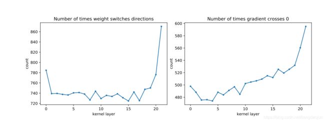
  The averages over the entire network are 741.9 for weight turns and 525.8 for gradients crossing zero. Note that the first and last layers oscillate more than their neighboring layers, which is interesting given that those layers hurt, but this is only a correlation as oscillations do not explain why something would bias towards helping or hurting.

参数和梯度在CIFAR-ResNet上的震荡（改变方向），可以比较一下权重和梯度的数量对比。下表是震荡的频率（震荡/迭代方向）：how often weight switches direction and how often gradient crosses zero.

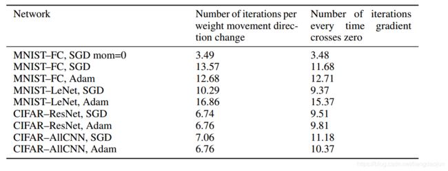
Noise persists across various hyperparameters.

Changing the learning rate, momentum, or batch size only have a slight effect on the percent of parameters helping. (表格 1)

Learning is heavy-tailed

A reasonable mental model of the distribution of LCA might be a narrow Gaussian around the mean. （图3（b））

Some layers hurt overall

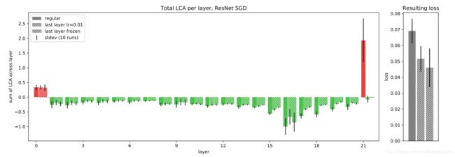
MNIST-FC 和LeNet的第一层和最后一层总是有害的！

Freezing the first layer stops it from hurting but causes others to help less.

左图：LCA 对整个训练过程中的每一层的和，CIFAR–Resnet的SGD 。偏置层和批范数层被合并到它们对应的核层中。蓝色表示正常的运行配置，其他颜色显示第一层上的各种实验。当第一层使用比其他层（橙色）小10倍的学习率时，每层LCA变化不大。虽然“第一层冻结”运行（绿色）在第一层中不再受影响（因为层参数从一开始就被冻结），但其他层，尤其是下两层，没有那么大帮助。当我们将第一层的lca argmin（红色）冻结时，也会看到类似的效果；当我们强制第一层的 LCA 为负时，其他层的 LCA 稍微为正，从而取消任何改进。中间：每次运行配置和标准偏差造成的训练损失。右图：第一层学习的典型累积轨迹，它在最初的几百次迭代中起到帮助作用，然后越来越有害。“在最小化冻结第一层”允许该层在冻结之前先提供帮助，但这仍然不能提高性能。

Freezing the last layer results in significant improvement.

Decreasing the learning rate of the last layer by 10x (0.01 as opposed to 0.1 for other layers) results in similar behavior as freezing it. These experiments are consistent with findings in [12] and [8], which demonstrate that you can freeze the last layer in some networks without degrading performance. With LCA, we are now able to provide an explanation for when and why this phenomenon happens. The instability of the last layer at the start of training can also be measured by LCA, as the LCA of the last layer is typically high in the first few iterations.

将最后一层的学习率降低10倍（0.01而不是其他层的0.1），会导致与冻结它类似的行为。这些实验与[12]和[8]中的研究结果一致，这表明您可以冻结某些网络中的最后一层，而不会降低性能。通过生命周期评价，我们现在能够解释这种现象发生的时间和原因。最后一层在训练开始时的不稳定性也可以用 LCA 来衡量，因为最后一层的 LCA 在前几次迭代中通常很高。

As the last layer helps more, the other layers hurt more because they are relatively more delayed. LCA of the last layer is fairly linear with respect to the delay.
由于最后一层的帮助更大，其他层的伤害也更大，因为它们相对延迟的时间更长。最后一层的 LCA 相对于延迟是相当线性的。

Phase shift hypothesis

相移假说

is the last layer phase-lagged?

最后一层时相移滞后吗？
min-batch 梯度是整个数据集梯度的无偏估计，所以需要从学习率和噪声之外寻找解释：我们假设最后一层的是相位滞后的，就是当所有层都震荡时，最后一层有点滞后。

We hypothesize that the last layer may be phase lagged with respect to other layers
during learning. Intuitively, it may be that while all layers are oscillating during learning, the last layer is always a bit behind. As each parameter swings back and forth across its valley, the shape of its valley is affected by the motion of all other parameters.
我们假设最后一层可能相对于其他层是相位滞后的。在学习过程中。直观地说，当学习过程中所有层都在振荡时，最后一层总是有点落后。当每个参数在山谷中来回摆动时，山谷的形状受所有其他参数的运动影响。

If one parameter is frozen and all other parameters trained infinitesimally slowly, that parameters valley will tend to flatten out. This means if it had climbed a valley (hurting the loss), it will not be able to fully recover the LCA in the negative direction, as the steep region has been flattened. If the last layer reacts slower than others, its own valley walls may tend to be flattened before it can react.

如果一个参数被冻结，而所有其他参数都被无限缓慢地训练，那么参数谷将趋于平缓。这意味着，如果它爬上了一个山谷（伤害了损失），它将无法在负方向上完全 LCA，因为陡峭的区域已经被夷为平地。如果最后一层的反应比其他层慢，它自己的谷壁可能会在反应之前被夷为平地。

As we give the last layer an information freshness advantage, it begins to “steal progress” from other layers, eventually forcing the neighboring layers into positive LCA.
当我们给最后一层一个信息新鲜度优势时，它开始从其他层“窃取进度”，最终迫使相邻层进入正的 LCA (有害的)。

These results suggest that it may be profitable to view training as a fundamentally oscillatory process upon which much research in phase-space representations and control system design may come to bear.
这些结果表明，将训练视为一个基本振荡过程可能是有益的，在此基础上，许多相空间表示和控制系统设计的研究可能会产生作用。

CIFAR–AllCNN trained with Adam does not have any hurting layers. We note that layers hurting is not a universal phenomenon that will be observed in all networks, but when it does occur, LCA can identify it. By using LCA we may identify layers as potential candidates to freeze. Further, viewing training through the lens of information delay seems valid, which suggests that per-layer optimization adjustments may be beneficial.
CIFAR–AllCNN 所有与adam一起训练的cnn没有任何伤害层。我们注意到，层伤害并不是所有网络都能观察到的普遍现象，但当它发生时，LCA 可以识别它。通过使用 LCA，我们可以将层识别为要冻结的潜在候选层。此外，从信息延迟的角度来看训练似乎是有效的，这表明逐层优化调整可能是有益的。

Learning is synchronized across layers

We learned that layers tend to have their own distinct, consistent behaviors regarding hurting or helping from per-layer LCA summed across all iterations.
我们了解到，在所有迭代中，每一层LCA都会对伤害或帮助产生不同的、一致的行为。

We further examine the per-layer LCA during training, equivalent to studying individual “loss curves” for each layer, and discover that the exact moments where learning peaks are curiously synchronized across layers. And such synchronization is not driven by only gradients or parameter motion, but both.
我们进一步研究了训练过程中的每一层 LCA，相当于研究每一层的个体“损失曲线”，并发现学习峰值的精确时刻在各层之间奇怪地同步。而且这种同步不是仅仅由梯度或参数运动驱动的，而是同时由两者驱动的。

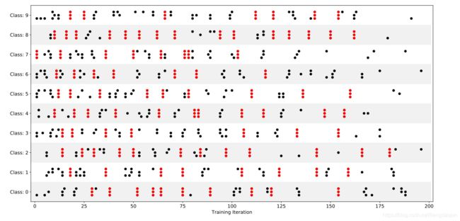
Peak learning iterations by layer by class on MNIST–FC. We define “moments of learning” as temporal spikes in an instantaneous LCA curve, local minima where loss decreased more on that iteration than on the iteration before or after, and show the top 20 such moments (highest magnitude of LCA) for each layer in above figure. We further decompose this metric by class (10 for both MNIST and CIFAR), where the same moments of learning are identified on per-class, per-layer LCAs, shown in above Figure. Whenever learning is synchronized across layers (dots that are vertically aligned) they are marked in red. The large proportion of red aligned stacks suggests that learning is very locally synchronized across layers.
我们将“学习时刻”定义为瞬时LCA曲线中的时间尖峰、局部极小值，其中该迭代的损失比迭代前后的损失减少更多，并在图S16中显示每层的前20个这样的时刻（LCA的最高值）。我们进一步分解这个按类度量（mnist和cifar均为10），其中在每类、每层lca上标识相同的学习时刻，如图6所示。每当学习跨层同步（垂直对齐的点）时，它们都被标记为红色。大量红色对齐的堆栈表明，学习是非常局部地跨层同步的。

We might find different behavior in other architectures such as transformer models or recurrent neural nets, which could be of interest for future work.

Appendix for this blog

Simpson’s Rule

  In Simpson’s Rule, we will use parabolas to approximate each part of the curve. This proves to be very efficient since it’s generally more accurate than the other numerical methods such as straight lines or trapezoid.

We divide the area into $n$ equal segments of width $\Delta x$. The approximate area is given by the following:

Note: In Simpson’s Rule, $n$ must be EVEN.
We can re-write Simpson’s Rule by grouping it as follows:

This gives us an easy way to remember Simpson’s Rule:

reference in here

Simpson法则的另一优点在于其自然引出了一种算法，即通过迭代使积分达到所需要的精确度。当积分的上下限相对于展开的中心点对称时，积分泰勒展开式中含有f(x)的奇数阶导数的项都将等于零。利用这一性质，我们可以在相邻的两个子区间内对面积作泰勒级数展开。

Runge-Kutta (RK4) Method

  The most point that need to illustrate is the RK4 method not appeared or explained in the original paper. So, you can skip this section if you feel it not necessary or useless. 原文中没又对 RK4 进行介绍，所以可以跳过该部分而不影响理解原文。

  The Runge-Kutta (RK4) methods are used to solve the solution of the non-liner ordinary differential equation. Here, we will simply summary this method.
  Assume the Intial Value Piont (IVP) is satisfied:
$$y\prime =f(t,y),y(t_0)=y_0(1)$$
  The formulation of RK4 is given by:
$$y_{(}n+1)=y_n+\frac{h}{6}(k_1+2k_2+2k_3+k_4)(2)$$
where, the $k_i$ represent the slope of middle points of the variable time $t$. Will, the Runge-Kutta methods just be generalized by RK4.