【图像识别】CIFAR-10（CNN）

一、CIFAR-10简介

CIFAR-10官网

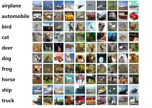
CIFAR-10 是由 Hinton的学生Alex Krizhevsky和 Ilya Sutskever 整理的一个用于识别普适物体的小型数据集。
它一共包含10个类别的RGB彩色图片，具体参考如下图：

数据集中一共有5000张训练图片和1000张测试图片，图片的尺寸大小为 32 * 32。

官方提供文件介绍：

文件	用途
cifar10.py	建立 CIFAR-10 预测模型
cifar10_input.py	在 TensorFlow 中读入 CIFAR-10 文件
cifar10_input_test.py	cifar10_input.py 的测试用例文件
cifar10_train.py	使用单个GPU或CPU训练模型
cifar10_train_multi_gpu.py	使用多个GPU训练模型
cifar10_eval.py	在测试集上测试模型的性能

- cifar10.py 文件中的 inference(images) 函数是官方提供的模型。 

二、CIFAR-10 和 MNIST数据集的区别

	CIFAR-10	MNIST
图像通道数	3 通道的 RGB 图像	灰度图像
尺寸大小	32 × 32	28 × 28
图片内容	现实世界的真实物体	0 ~ 9 数字
图片特点	噪声很大，可能有背景图片或其他物体干扰； 物体的比例、特征都不尽相同，识别难度大	噪声小，干扰物体少； 易识别

 三、参考官方代码编写CNN模型

import tensorflow as tf
import numpy as np
import time
import math
# 官方提供的两个文件，用于对数据集的输入等操作
import cifar10
import cifar10_input

max_steps = 3000 # 训练次数
batch_size = 128 # 批处理参数

# ---1.加载数据 ---

# 下载cifar10数据集的默认路径，需要把cifar10.py/line 53/对应代码改一下
data_dir = 'D:/Python_code/Data/cifar-10-python/cifar-10-batches-bin'

# 权值初始化函数（shape，标准差，L2正则化比例系数）
def variable_with_weight_losses(shape, stddev, wl):
  # 使用tf.truncated_normal截断的正态分布来初始化
  var = tf.Variable(tf.truncated_normal(shape, stddev=stddev))
  if wl is not None:
    # 做一个L2的正则化处理，用wl控制L2的大小比例
    weight_loss = tf.multiply(tf.nn.l2_loss(var), wl, name='weight_loss')
    # 将weight_loss统一存放起来
    tf.add_to_collection("losses", weight_loss)
  return var

# 调用cifar10.py中的一个函数，下载数据集，并解压
cifar10.maybe_download_and_extract()

# 生成训练数据，使用distorted_inputs函数，做数据增强处理
images_train, labels_train = cifar10_input.distorted_inputs(data_dir=data_dir, batch_size=batch_size)
# 生成测试数据，不必做数据增强
images_test, labels_test = cifar10_input.inputs(eval_data=True, data_dir=data_dir, batch_size=batch_size)

# 占位符
image_holder = tf.placeholder(tf.float32, [batch_size, 24, 24, 3])
label_holder = tf.placeholder(tf.int32, [batch_size])


# ---2. 构建模型 ---

# 第一层卷积层，64个卷积核，大小为5*5，3通道（RGB三种颜色通道）
  # 1).定义权重
weight1 = variable_with_weight_losses(shape=[5,5,3,64], stddev=0.05, wl=0.0)
  # 2).卷积操作
kernel1 = tf.nn.conv2d(image_holder, filter=weight1, strides=[1, 1, 1, 1], padding='SAME')
  # 3).定义偏差
bias1 = tf.Variable(tf.constant(0.0, shape=[64]))
  # 4).relu激活函数
conv1 = tf.nn.relu(tf.nn.bias_add(kernel1, bias1))
  # 5).最大池化
pool1 = tf.nn.max_pool(conv1, ksize=[1, 3, 3, 1], strides=[1, 2, 2, 1], padding='SAME')
  # 6.lrn: 局部响应归一化，可防止过拟合，原理是生物学上的‘侧抑制’，（通俗来讲就是增强强的地方，削弱弱的地方）
  # pool1表示输入数据，4表示使用前后几层进行归一化操作，bias表示偏移量，alpha和beta表示系数
norm1 = tf.nn.lrn(pool1, 4, bias=1.0, alpha=0.001/9.0, beta=0.75)

# 第二层卷积层
weight2 = variable_with_weight_losses(shape=[5,5,64,64], stddev=5e-2, wl=0.0)
kernel2 = tf.nn.conv2d(norm1, filter=weight2, strides=[1, 1, 1, 1], padding='SAME')
bias2 = tf.Variable(tf.constant(0.1, shape=[64]))
conv2 = tf.nn.relu(tf.nn.bias_add(kernel2, bias2))
norm2 = tf.nn.lrn(conv2, 4, bias=1.0, alpha=0.001/9.0, beta=0.75)
pool2 = tf.nn.max_pool(norm2, ksize=[1, 3, 3, 1], strides=[1, 2, 2, 1], padding='SAME')

# 第三层全连接层
# 将第二层卷积层输出结果变成一维向量
reshape = tf.reshape(pool2, [batch_size, -1])
dim = reshape.get_shape()[1].value
# 初始化权值，隐含节点384个，正态分布标准差为0.04，偏差bias为0.1
weight3 = variable_with_weight_losses(shape=[dim,384], stddev=0.04, wl=0.004)
bias3 = tf.Variable(tf.constant(0.1, shape=[384]))
local3 = tf.nn.relu(tf.matmul(reshape, weight3) + bias3)

# 第四层全连接层
weight4 = variable_with_weight_losses(shape=[384,192], stddev=0.04, wl=0.004)
bias4 = tf.Variable(tf.constant(0.1, shape=[192]))
local4 = tf.nn.relu(tf.matmul(local3, weight4) + bias4)

# 第五层输出层
weight5 = variable_with_weight_losses(shape=[192,10], stddev=1/192.0, wl=0.0)
bias5 = tf.Variable(tf.constant(0.0, shape=[10]))
logits = tf.add(tf.matmul(local4, weight5), bias5)

# 定义损失函数
def loss(logits, labels):
  labels = tf.cast(labels, tf.int64)
  # 交叉熵损失函数
  cross_entropy = tf.reduce_mean(tf.nn.sparse_softmax_cross_entropy_with_logits(
    logits=logits, labels=labels
  ))
  tf.add_to_collection('losses', cross_entropy)
  return tf.add_n(tf.get_collection('losses'), name='total_loss')

loss = loss(logits=logits,labels=label_holder)
train_op = tf.train.AdamOptimizer(0.001).minimize(loss)
top_k_op = tf.nn.in_top_k(logits, label_holder, 1)

# ---3. 训练模型---
sess = tf.InteractiveSession()
tf.global_variables_initializer().run()
# 引入多线程
tf.train.start_queue_runners()

for step in range(max_steps):
  start_time = time.time()
  image_batch, label_batch = sess.run([images_train, labels_train])
  _, loss_value = sess.run([train_op, loss], feed_dict={image_holder: image_batch, label_holder: label_batch})
  duration = time.time() - start_time
  if step % 10 == 0:
    examples_per_sec = batch_size / duration
    sec_per_batch = float(duration)
    str = 'step %d, loss = %.2f (%.1f examples/sec; %.3f sec/batch)'
    #print(step, loss_value)
    print(str % (step, loss_value, examples_per_sec, sec_per_batch))

num_examples = 10000
num_iter = int(math.ceil(num_examples / batch_size))
true_count = 0
total_sample_count = num_iter * batch_size
step = 0
while step < num_iter:
  image_batch, label_batch = sess.run([images_test, labels_test])
  predictions = sess.run([top_k_op], feed_dict={image_holder: image_batch, label_holder: label_batch})
  true_count += np.sum(predictions)
  step += 1

precision = true_count / total_sample_count
print('precision = %.3f' % precision)

 

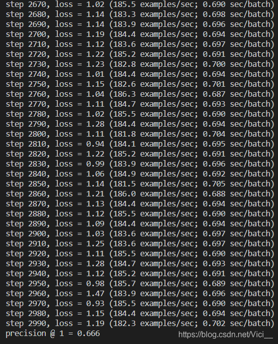
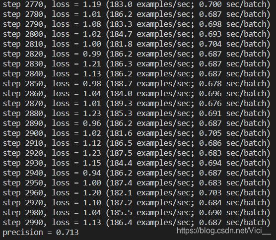
四、训练结果

左图是基于 MNIST 采用 RMSProp 算法的优化器；
右图是参考书籍采用 Adam 优化器。
测试次数都是3000次。

   

 

参考文献：

1. 《21个项目玩转深度学习》何之源 
2.    bilibili - CNN识别图片
3.    CIFAR 官网