数值分析实验一(线性方程组的求解 基于matlab实现)

Jacobi Method

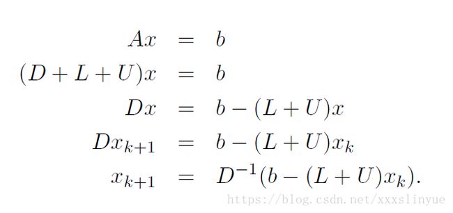
The Jacobi Method is a form of fixed-point iteration. Let D denote the main diagonal

of A, L denote the lower triangle of A (entries below the main diagonal), and U denote the

upper triangle (entries above the main diagonal). Then A = L + D + U, and the equation

to be solved is Lx + Dx + Ux = b. Note that this use of L and U differs from the use

in the LU factorization, since all diagonal entries of this L and U are zero. The system of

equations Ax = b can be rearranged in a fixed-point iteration of form:

function [x]=jacobi(A,x0,b)
D=diag(diag(A));
L=tril(A,-1);
U=triu(A,1);
B=-inv(D)*(L+U);
g=inv(D)*b;
for i=1:15
    x=B*x0+g;
    x0=x;
end

 

Gauss–Seidel Method:

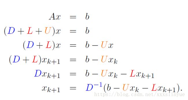
Closely related to the Jacobi Method is an iteration called the Gauss–Seidel Method. The

only difference between Gauss–Seidel and Jacobi is that in the former, the most recently

updated values of the unknowns are used at each step, even if the updating occurs in the

current step.

function [x]=gauss(A,x0,b)
D=diag(diag(A)); 
L=tril(A,-1);   
U=triu(A,1);
B = -inv(D+L)*U;
g = inv(D+L)*b; 
for k=1:15
    x=B*x0+g;
    x0=x;
end

 

Successive Over-Relaxation Method:

The method called Successive Over-Relaxation (SOR) takes the Gauss–Seidel direc-

tion toward the solution and “overshoots’’ to try to speed convergence. Let ω be a real number, and define each component of the new guess x k+1 as a weighted average of ω

times the Gauss–Seidel formula and 1 − ω times the current guess x k . The number ω is

called the relaxation parameter, and ω > 1 is referred to as over-relaxation.

(L+D+U)x=b

 

function [x]=sor(A,x0,b,w)
D=diag(diag(A)); 
L=tril(A,-1);  
U=triu(A,1);
B = inv(D+w*L)*((1-w)*D-w*U);
g = w*inv(D+w*L)*b;
for k=1:15
    x=B*x0+g;
    x0=x;
end

Conjugate Gradient Method;

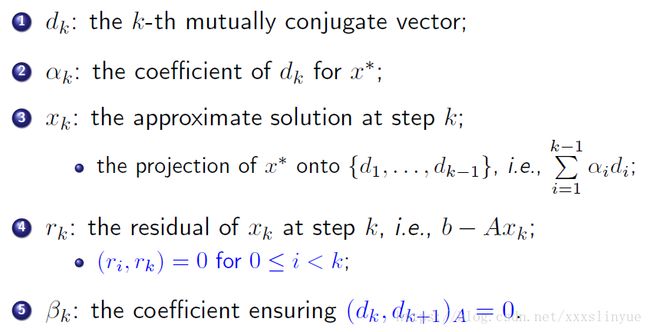
So,

 

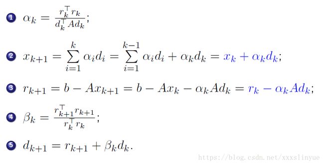
function [x0]=conjugate(A,x0,b)
d0 = b-(A*x0);
r0 = d0;
for k=1:15
    a = (norm(r0))^2/(d0'*A*d0); 
    x0 = x0+a*d0; 
    r1 = r0-a*A*d0;
    beta = (norm(r1)^2)/(norm(r0)^2);
    d0 = r1+beta*d0;
    r0 = r1;
end

 

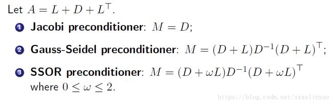
Conjugate Gradient Method with Jacobi preconditioner.

 

 

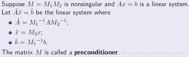
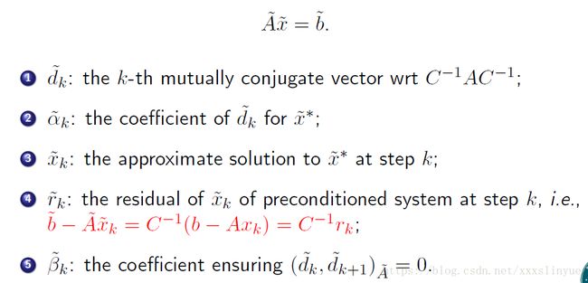
Then:

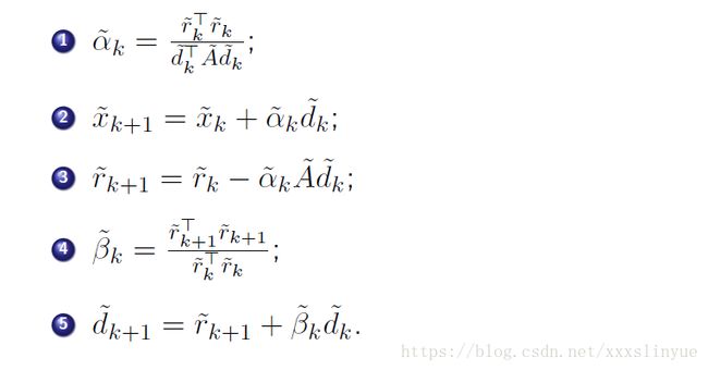
function [x0]=preconditionConjugate(A,x0,b)
D = diag(diag(A));
M = D;
r0 = b-(A*x0);
z0 = inv(M)*r0;
d0 = z0;
for k=1:15  
    a = (r0'*z0)/(d0'*A*d0); 
    x0 = x0+a*d0;
    r1 = r0-a*A*d0;
    z1 = inv(M)*r1;
    beta = (r1'*z1)/(r0'*z0);
    d0 = r1+beta*d0;
    r0 = r1; z0 = z1;
end