用R进行相关分析及其制图可视化

1 R基础包stats里的cor函数
R代码如下:
options(digits=2)
library(RSTAT2D); data('d5.8.1.1')
df <- d5.8.1.1[,-1]
cov(df)
cor(df)
cor(df, method = "spearman")
运行结果如下:
> cov(df)
           h    dbh       v   cpro      wd    wpro     tl      tw     lrt
h       2.88    8.1   0.416   -6.8   -21.6    23.6   -114  -0.201   -2.22
dbh     8.09   30.6   1.483  -21.2   -86.0    94.1   -325  -2.653   -3.13
v       0.42    1.5   0.074   -1.1    -4.6     5.1    -18  -0.098   -0.25
cpro   -6.78  -21.2  -1.089   86.4    90.6  -101.2    538  -2.208   14.62
wd    -21.64  -86.0  -4.589   90.6  1939.4 -1876.2  -1256 -11.655   -1.20
wpro   23.64   94.1   5.093 -101.2 -1876.2  1892.9    284  -2.278    3.12
tl   -114.11 -324.9 -17.919  538.2 -1255.7   284.1 109016 170.587 2071.07
tw     -0.20   -2.7  -0.098   -2.2   -11.7    -2.3    171  10.016  -11.74
lrt    -2.22   -3.1  -0.250   14.6    -1.2     3.1   2071 -11.741   62.60

> cor(df) # 计算pearson相关系数
          h    dbh     v   cpro      wd    wpro     tl     tw     lrt
h     1.000  0.862  0.90 -0.430 -0.2896  0.3202 -0.204 -0.037 -0.1650
dbh   0.862  1.000  0.98 -0.413 -0.3529  0.3908 -0.178 -0.152 -0.0715
v     0.900  0.984  1.00 -0.430 -0.3825  0.4297 -0.199 -0.113 -0.1161
cpro -0.430 -0.413 -0.43  1.000  0.2214 -0.2503  0.175 -0.075  0.1988
wd   -0.290 -0.353 -0.38  0.221  1.0000 -0.9793 -0.086 -0.084 -0.0035
wpro  0.320  0.391  0.43 -0.250 -0.9793  1.0000  0.020 -0.017  0.0091
tl   -0.204 -0.178 -0.20  0.175 -0.0864  0.0198  1.000  0.163  0.7928
tw   -0.037 -0.152 -0.11 -0.075 -0.0836 -0.0165  0.163  1.000 -0.4689
lrt  -0.165 -0.071 -0.12  0.199 -0.0035  0.0091  0.793 -0.469  1.0000

> cor(df, method = "spearman") # 计算spearman相关系数
          h   dbh     v  cpro     wd   wpro     tl     tw    lrt
h     1.000  0.81  0.90 -0.20 -0.218  0.218 -0.214 -0.051 -0.132
dbh   0.812  1.00  0.98 -0.22 -0.296  0.296 -0.206 -0.267  0.020
v     0.900  0.98  1.00 -0.24 -0.263  0.263 -0.208 -0.188 -0.030
cpro -0.202 -0.22 -0.24  1.00  0.168 -0.168  0.215 -0.060  0.225
wd   -0.218 -0.30 -0.26  0.17  1.000 -1.000  0.087  0.165 -0.032
wpro  0.218  0.30  0.26 -0.17 -1.000  1.000 -0.087 -0.165  0.032
tl   -0.214 -0.21 -0.21  0.22  0.087 -0.087  1.000  0.257  0.755
tw   -0.051 -0.27 -0.19 -0.06  0.165 -0.165  0.257  1.000 -0.362
lrt  -0.132  0.02 -0.03  0.22 -0.032  0.032  0.755 -0.362  1.000
相关显著性的检验

R代码和结果如下:
> cor.test(df[,3], df[,5])
 Pearson's product-moment correlation
data:  df[, 3] and df[, 5]
t = -2, df = 30, p-value = 0.04
alternative hypothesis: true correlation is not equal to 0
95 percent confidence interval:
 -0.653 -0.026
sample estimates:
  cor
-0.38
> cor.test(df[,3], df[,5], method = "spearman")
 Spearman's rank correlation rho
data:  df[, 3] and df[, 5]
S = 6000, p-value = 0.2
alternative hypothesis: true rho is not equal to 0
sample estimates:
  rho
-0.26
但cor.test()每次只能检验一个相关的显著性。
2 agricolae包的correlation函数
> library(agricolae)
> correlation(df, method="pearson")
Correlation Analysis

Method     : pearson
Alternative: two.sided

$correlation
         h   dbh     v  cpro    wd  wpro    tl    tw   lrt
h     1.00  0.86  0.90 -0.43 -0.29  0.32 -0.20 -0.04 -0.17
dbh   0.86  1.00  0.98 -0.41 -0.35  0.39 -0.18 -0.15 -0.07
v     0.90  0.98  1.00 -0.43 -0.38  0.43 -0.20 -0.11 -0.12
cpro -0.43 -0.41 -0.43  1.00  0.22 -0.25  0.18 -0.08  0.20
wd   -0.29 -0.35 -0.38  0.22  1.00 -0.98 -0.09 -0.08  0.00
wpro  0.32  0.39  0.43 -0.25 -0.98  1.00  0.02 -0.02  0.01
tl   -0.20 -0.18 -0.20  0.18 -0.09  0.02  1.00  0.16  0.79
tw   -0.04 -0.15 -0.11 -0.08 -0.08 -0.02  0.16  1.00 -0.47
lrt  -0.17 -0.07 -0.12  0.20  0.00  0.01  0.79 -0.47  1.00

$pvalue
           h     dbh       v  cpro    wd  wpro      tl    tw     lrt
h    1.0e+00 9.2e-10 1.3e-11 0.018 0.121 0.084 2.8e-01 0.844 3.8e-01
dbh  9.2e-10 1.0e+00 0.0e+00 0.023 0.056 0.033 3.5e-01 0.424 7.1e-01
v    1.3e-11 0.0e+00 1.0e+00 0.018 0.037 0.018 2.9e-01 0.551 5.4e-01
cpro 1.8e-02 2.3e-02 1.8e-02 1.000 0.240 0.182 3.5e-01 0.693 2.9e-01
wd   1.2e-01 5.6e-02 3.7e-02 0.240 1.000 0.000 6.5e-01 0.660 9.9e-01
wpro 8.4e-02 3.3e-02 1.8e-02 0.182 0.000 1.000 9.2e-01 0.931 9.6e-01
tl   2.8e-01 3.5e-01 2.9e-01 0.354 0.650 0.917 1.0e+00 0.389 1.8e-07
tw   8.4e-01 4.2e-01 5.5e-01 0.693 0.660 0.931 3.9e-01 1.000 9.0e-03
lrt  3.8e-01 7.1e-01 5.4e-01 0.292 0.986 0.962 1.8e-07 0.009 1.0e+00

$n.obs
[1] 30
3 psych包的corr.test函数
> library(psych) ; corr.test(df, use = "complete")
Call:corr.test(x = df, use = "complete")
Correlation matrix
         h   dbh     v  cpro    wd  wpro    tl    tw   lrt
h     1.00  0.86  0.90 -0.43 -0.29  0.32 -0.20 -0.04 -0.17
dbh   0.86  1.00  0.98 -0.41 -0.35  0.39 -0.18 -0.15 -0.07
v     0.90  0.98  1.00 -0.43 -0.38  0.43 -0.20 -0.11 -0.12
cpro -0.43 -0.41 -0.43  1.00  0.22 -0.25  0.18 -0.08  0.20
wd   -0.29 -0.35 -0.38  0.22  1.00 -0.98 -0.09 -0.08  0.00
wpro  0.32  0.39  0.43 -0.25 -0.98  1.00  0.02 -0.02  0.01
tl   -0.20 -0.18 -0.20  0.18 -0.09  0.02  1.00  0.16  0.79
tw   -0.04 -0.15 -0.11 -0.08 -0.08 -0.02  0.16  1.00 -0.47
lrt  -0.17 -0.07 -0.12  0.20  0.00  0.01  0.79 -0.47  1.00
Sample Size
[1] 30
Probability values (Entries above the diagonal are adjusted for multiple tests.)
        h  dbh    v cpro   wd wpro   tl   tw  lrt
h    0.00 0.00 0.00 0.53 1.00 1.00 1.00 1.00 1.00
dbh  0.00 0.00 0.00 0.63 1.00 0.85 1.00 1.00 1.00
v    0.00 0.00 0.00 0.53 0.92 0.53 1.00 1.00 1.00
cpro 0.02 0.02 0.02 0.00 1.00 1.00 1.00 1.00 1.00
wd   0.12 0.06 0.04 0.24 0.00 0.00 1.00 1.00 1.00
wpro 0.08 0.03 0.02 0.18 0.00 0.00 1.00 1.00 1.00
tl   0.28 0.35 0.29 0.35 0.65 0.92 0.00 1.00 0.00
tw   0.84 0.42 0.55 0.69 0.66 0.93 0.39 0.00 0.28
lrt  0.38 0.71 0.54 0.29 0.99 0.96 0.00 0.01 0.00
注意: corr.test函数可对相关显著检验进行多重校正,提高检验的严谨性。
4 correlation包的correlation函数
> library(dplyr)
> library(correlation)
> df %>% correlation::correlation() %>% summary
  Parameter |     lrt |    tw |    tl |     wpro |    wd |  cpro |       v |     dbh
  ----------------------------------------------------------------------------------
  h         |   -0.17 | -0.04 | -0.20 |     0.32 | -0.29 | -0.43 | 0.90*** | 0.86***
  dbh       |   -0.07 | -0.15 | -0.18 |     0.39 | -0.35 | -0.41 | 0.98*** |
  v         |   -0.12 | -0.11 | -0.20 |     0.43 | -0.38 | -0.43 |         |
  cpro      |    0.20 | -0.08 |  0.18 |    -0.25 |  0.22 |       |         |
  wd        |    0.00 | -0.08 | -0.09 | -0.98*** |       |       |         |
  wpro      |    0.01 | -0.02 |  0.02 |          |       |       |         |
  tl        | 0.79*** |  0.16 |       |          |       |       |         |
  tw        |   -0.47 |       |       |          |       |       |         |
5 相关关系的可视化
5.1 corrgram包
library(corrgram)
corrgram(df, order=T, lower.panel=panel.shade,
         upper.panel=panel.pie, text.panel=panel.txt,
         main="Correlogram of fir traits")

order参数的优点:可以对变量的相关关系进行聚类分析,了解变量间的归属关系。
5.2 qgraph包
library(dplyr)
library(qgraph)
df %>% cor() %>% qgraph()

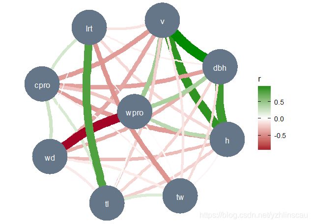
5.3 see包
library(correlation)
library(see)
library(ggraph)
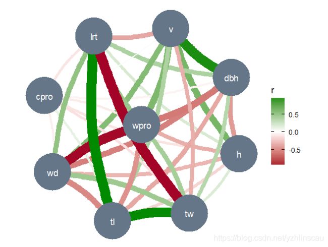
df %>% correlation() %>% plot
加入偏相关参数
df %>% correlation(partial=TRUE) %>% plot
除了上述介绍的简单相关外,还有偏相关、复相关和典型相关等。