CMU 11-785 L16 Connectionist Temporal Classification

Sequence to sequence

• Sequence goes in, sequence comes out
• No notion of “time synchrony” between input and output
  • May even nots maintain order of symbols (from one language to another)

With order synchrony

• The input and output sequences happen in the same order
  • Although they may be time asynchronous
  • E.g. Speech recognition
    • The input speech corresponds to the phoneme sequence output
• Question
  • How do we know when to output symbols
  • In fact, the network produces outputs at every time
  • Which of these are the real outputs?

Option 1

• Simply select the most probable symbol at each time
• Merge adjacent repeated symbols, and place the actual emission of the symbol in the final instant
• Problem
  • Cannot distinguish between an extended symbol and repetitions of the symbol
  • Resulting sequence may be meaningless

Option 2

• Impose external constraints on what sequences are allowed
  • E.g. only allow sequences corresponding to dictionary words

Decoding

• The process of obtaining an output from the network

• Time-synchronous & order-synchronous sequence

  • aaabbbbbbccc => abc (probility 0.5)
    aabbbbbbbccc => abc (probility 0.001)
    cccddddddeee => cde (probility 0.4)
    cccddddeeeee => cde (probility 0.4)
    

  • So abc is the most likely time-synchronous output sequence
  • But cde is the the most likely order-synchronous sequence

• Option 2 is in fact a suboptimal decode that actually finds the most likely time-synchronous output sequence

• The “merging” heuristics do not guarantee optimal order-synchronous sequences

No timing information provided

• Only the sequence of output symbols is provided for the training data
  • But no indication of which one occurs where

Guess the alignment

• Initialize
  • Assign an initial alignment
  • Either randomly, based on some heuristic, or any other rationale
• Iterate
  • Train the network using the current alignment
  • Reestimate the alignment for each training instance

Constraining the alignment

• Try 1
  • Block out all rows that do not include symbols from the target sequence
  • E.g. Block out rows that are not /B/ /IY/ or /F/
• Only decode on reduced grid
  • We are now assured that only the appropriate symbols will be hypothesized
• But this still doesn’t assure that the decode sequence correctly expands the target symbol sequence
  • Order variance
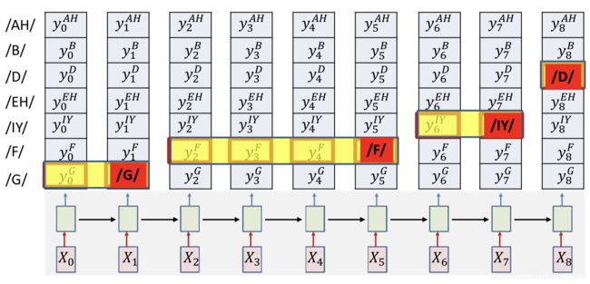
• Try 2
  • Explicitly arrange the constructed table
  • Arrange the constructed table so that from top to bottom it has the exact sequence of symbols required
    • If a symbol occurs multiple times, we repeat the row in the appropriate location

• Constrain that the first symbol in the decode must be the top left block

  • The last symbol must be the bottom right
  • The rest of the symbols must follow a sequence that monotonically travels down from top left to bottom right
  • This guarantees that the sequence is an expansion of the target sequence

• Compose a graph such that every path in the graph from source to sink represents a valid alignment

  • The “score” of a path is the product of the probabilities of all nodes along the path
  • Find the most probable path from source to sink using any dynamic programming algorithm (viterbi algorithm)

Viterbi algorithm

• Main idea

  • The best path to any node must be an extension of the best path to one of its parent nodes

• Dynamically track the best path (and the score of the best path) from the source node to every node in the graph

  • At each node, keep track of
    • The best incoming parent edge (BP)
    • The score of the best path from the source to the node through this best parent edge (Bscr)

• Process
  

• Algorithm
  

Gradients

$$DIV=\sum _{t}Xent\left(Y_t,symbo{l}_t^{bestpath}\right)=-\sum _t\log Y\left(t,symbo{l}_t^{bestpath}\right)$$

• The gradient w.r.t the -th output vector $Y_t$
  $${\nabla }_{Y_t}DIV=[00\cdot \cdot \cdot \frac{-1}{Y(t,symbo{l}_t^{bestpath})}0\cdot \cdot \cdot 0]$$

• Problem

  • Approach heavily dependent on initial alignment
  • Prone to poor local optima
    • Because we commit to the single “best” estimated alignment
    • This can be way off, particularly in early iterations, or if the model is poorly initialized

• Alternate view

  • There is a probability distribution over alignments of the target Symbol sequence (to the input)
  • Selecting a single alignment is the same as drawing a single sample from it

• Instead of only selecting the most likely alignment, use the statistical expectation over all possible alignments

  • $$DIV=E\left[-\sum _t\log Y\left(t,s_t\right)\right]$$

  • Use the entire distribution of alignments

  • This will mitigate the issue of suboptimal selection of alignment

• Using the linearity of expectation

  • $$DIV=-\sum _{t}E\left[\log Y\left(t,s_t\right)\right]$$

  • $$DIV=-\sum _t\sum _{S\in S_1\dots S_K}P\left(s_t=S|\mathbf{S},\mathbf{X}\right)\log Y\left(t,s_t=S\right)$$

A posteriori probabilities of symbols

• $P(s_t=S|\mathbf{S},\mathbf{X})$ is the probability of seeing the specific symbol $s$ at time $t$, given that the symbol sequence is an expansion of $S=s_0,...,S_{K-1}$ and given the input sequence $X=X_o,...,X_{N-1}$

  • $P\left(s_t=S_r|\mathbf{S},\mathbf{X}\right)\propto P\left(s_t=S_r,\mathbf{S}|\mathbf{X}\right)$

• $P\left(s_t=S_r,\mathbf{S}|\mathbf{X}\right)$ is the total probability of all valid paths in the graph for target sequence $S$ that go through the symbol $S_r$ (the $r^{th}$ symbol in the sequence $S_0,...,S_{K-1}$ ) at time

• For a recurrent network without feedback from the output we can make the conditional independence assumption

$$P\left(s_t=S_r,\mathbf{S}|\mathbf{X}\right)=P\left(S_0\dots S_r,s_t=S_r|\mathbf{X}\right)P\left(s_{t+1}\in \mathrm{succ}\left(S_r\right),\mathrm{succ}\left(S_r\right),\dots ,S_{K-1}|\mathbf{X}\right)$$

• We will call the first term the forward probability $\alpha (t,r)$
• We will call the second term the backward probability $\beta (t,r)$

Forward algorithm

• In practice the recursion will gererally underflow

$$\alpha (t,l)=(\alpha (t-1,l)+\alpha (t-1,l-1))y_t^{S(l)}$$

• Instead we can do it in the log domain

$$\log \alpha (t,l)=\log \left(e^{\log \alpha (t-1,l)}+e^{\log \alpha (t-1,l-1)}\right)+\log y_t^{S(l)}$$

Backward algorithm

$$\beta (t,r)=P\left(s_{t+1}\in \mathrm{succ}\left(S_r\right),\mathrm{succ}\left(S_r\right),\dots ,S_{K-1}|\mathbf{X}\right)$$

The joint probability

$$P\left(s_t=S_r,\mathbf{S}|\mathbf{X}\right)=\alpha (t,r)\beta (t,r)$$

• Need to be normalized, get posterior probability

$$\gamma (t,r)=P\left(s_t=S_r|\mathbf{S},\mathbf{X}\right)=\frac{P\left(s_t=S_r,\mathbf{S}|\mathbf{X}\right)}{{\sum }_{S_r^{\prime }}P\left(s_t=S_r^{\prime },\mathbf{S}|\mathbf{X}\right)}=\frac{\alpha (t,r)\beta (t,r)}{{\sum }_{r^{\prime }}\alpha \left(t,r^{\prime }\right)\beta \left(t,r^{\prime }\right)}$$

• We can also write this using the modified beta formula as (you will see this in papers)

$$\gamma (t,r)=\frac{\frac{1}{y_t^{S(r)}}\alpha (t,r)\hat{\beta }(t,r)}{{\sum }_{r^{\prime }}\frac{1}{y_t^{S(r)}}\alpha (t,r)\hat{\beta }(t,r)}$$

The expected divergence

$$DIV=-\sum _t\sum _{s\in S_0\dots S_{K-1}}P\left(s_t=s|\mathbf{S},\mathbf{X}\right)\log Y\left(t,s_t=s\right)$$

$$DIV=-\sum _t\sum _r\gamma (t,r)\log y_t^{S(r)}$$

• The derivative of the divergence w.r.t the output $Y_t$ of the net at any time

$${\nabla }_{Y_t}DIV=\left[\begin{array}{llll}\frac{dDIV}{d{y}_t^{S_0}}& \frac{dDIV}{d{y}_t^{S_1}}& \cdots & \frac{dDIV}{d{y}_t^{S_{L-1}}}\end{array}\right]$$

• Compare to Viterbi algorithm, components will be non-zero only for symbols that occur in the training instance

• Compute derivative

$$\frac{dDIV}{d{y}_t^l}=-\sum _{r:S(r)=l}\frac{d}{d{y}_t^{S(r)}}\gamma (t,r)\log y_t^{S(r)}$$

$$\frac{d}{d{y}_t^{S(r)}}\gamma (t,r)\log y_t^{S(r)}=\frac{\gamma (t,r)}{y_t^{S(r)}}+\frac{d\gamma (t,r)}{d{y}_t^{S(r)}}\log y_t^{S(r)}$$

• Normally we ignore the second term, and think of as a maximum-likelihood estimate
• And the derivatives at both these locations must be summed if occurs repetition

$$\frac{dDIV}{d{y}_t^l}=-\sum _{r:S(r)=l}\frac{\gamma (t,r)}{y_t^{S(r)}}$$

Repetitive decoding problem

• Cannot distinguish between an extended symbol and repetitions of the symbol
  • We have a decode: R R R O O O O O D
  • Is this the symbol sequence ROD or ROOD?
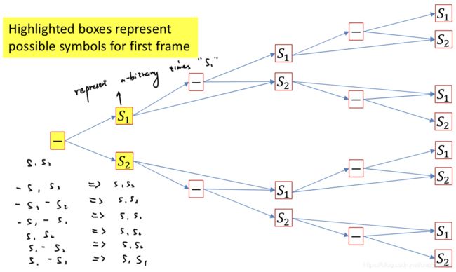
• Solution: Introduce an explicit extra symbol which serves to separate discrete versions of a symbol
  • A “blank” (represented by “-”)
  • RRR—OO—DDD = ROD
  • RR-R—OO—D-DD = RRODD

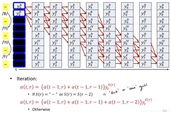
Modified forward algorithm

• A blank is mandatory between repetitions of a symbol but not required between distinct symbols
• Skips are permitted across a blank, but only if the symbols on either side are different

Modified backward algorithm

Overall training procedure

1. Setup the network

   • Typically many-layered LSTM

2. Initialize all parameters of the network

   • Include a 「blank」 symbol in vocabulary

3. Foreach training instance

   • Pass the training instance through the network and obtain all symbol probabilities at each time
   • Construct the graph representing the specific symbol sequence in the instance

4. Backword pass

   • Perform the forward backward algorithm to compute $\alpha (t,r)$ and $\beta (t,r)$

   • Compute derivative of divergence ${\nabla }_{Y_t}DIV$ for each $Y_t$

   • $${\nabla }_{Y_t}DIV=\left[\begin{array}{llll}\frac{dDIV}{d{y}_t^0}& \frac{dDIV}{d{y}_t^1}& \cdots & \frac{dDIV}{d{y}_t^{L-1}}\end{array}\right]$$

   • $$\frac{dDIV}{d{y}_t^l}=-\sum _{r:S(r)=l}\frac{\gamma (t,r)}{y_t^{S(r)}}$$

   • Aggregate derivatives over minibatch and update parameters

• CTC: Connectionist Temporal Classification
  • The overall framework is referred to as CTC
  • This is in fact a suboptimal decode that actually finds the most likely time-synchronous output sequence
• Actual decoding objective
  • $\hat{\mathbf{S}}=\underset{\mathbf{s}}{\mathrm{argmax}}{\alpha }_{\mathbf{S}}\left(S_{K-1},T-1\right)$
  • Explicit computation of this will require evaluate of an exponential number of symbol sequences

Beam search

• Only used in test
• Uses breadth-first search to build its search tree
  • Choose top k words for next prediction (prone)

• Reference