滤波器设计

Peak

code

% Loader Octave packages
pkg load signal

% Sample Rate
Fs = 48000;

% Designed by personal tool Math.exe
% Math.exe filter --design -t 3 -w 1000 -f 48000 -b 10.0 -g 0.0 -s 8.0
% Fs       : 48000
% Fc       : 1000
% Boost    : 10.0
% Gain     : 0.0
% Slope    : 8.0
A_PEAK = [+1.000000, -1.973835, +0.990867];
B_PEAK = [+1.009874, -1.973835, +0.980993];

% Generate response matrix that size is Fs.
[H_PEAK, w_PEAK] = freqz(B_PEAK, A_PEAK, Fs);

% Transfer from Rad to Hz.
F_PEAK = (w_PEAK / (2 * pi)) * Fs;

% Transfer from Magnitude to DB
Hf_PEAK = mag2db(abs(H_PEAK));
Hx_PEAK = angle(H_PEAK);

clear figure
clf;
figure(1);

% Plot Magnitude VS Frequency
% Range: 1 ~ (Fs / 6) / 2 = 1 ~ 4000
% Because Freqz only return half result (1, +pi) rather than (-pi, +pi),
% So divided by 2.
subplot(2, 1, 1);
plot(F_PEAK(1:Fs/6,1), Hf_PEAK(1:Fs/6,1));

% Plot Phase VS Frequency
subplot(2, 1, 2);
plot(F_PEAK(1:Fs/6,1), Hx_PEAK(1:Fs/6,1));

plot

DF_I

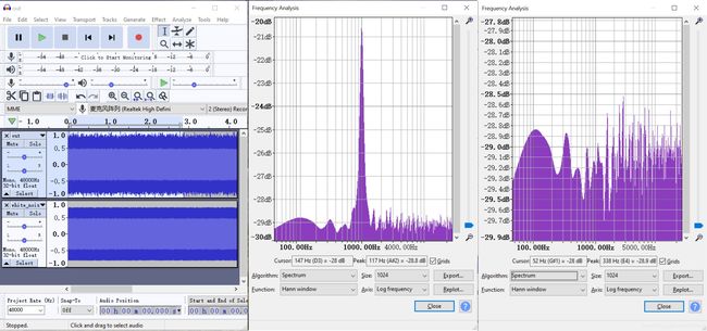
• 生成一个白噪音信号
• 进行Direct formal I Biquad处理
• 利用Audacity分析

注：
左图为经过处理的信号和源信号。
中图为经过处理的信号的频谱分析（FFT分析）
右图为经过源信号的频谱分析
通过上图，可以明显看见，滤波效果非常显著。

Pass

code

% Loader Octave packages
pkg load signal

% Sample Rate
Fs = 48000;

% Corner Frequency
F0 = 1000;
Wn = [(F0-100)/(Fs/2), (F0+100)/(Fs/2)];

[B_PASS, A_PASS] = butter(2, Wn, 'pass');
% Generate response matrix that size is Fs.
[H_PASS, w_PASS] = freqz(B_PASS, A_PASS, Fs);

% Transfer from Rad to Hz.
F_PASS = (w_PASS / (2 * pi)) * Fs;

% Transfer from Magnitude to DB
Hf_PASS = mag2db(abs(H_PASS));
Hx_PASS = angle(H_PASS);

clear figure
clf;
figure(1);

% Plot Magnitude VS Frequency
% Range: 1 ~ (Fs / 6) / 2 = 1 ~ 4000
% Because Freqz only return half result (1, +pi) rather than (-pi, +pi),
% So divided by 2.
subplot(2, 1, 1);
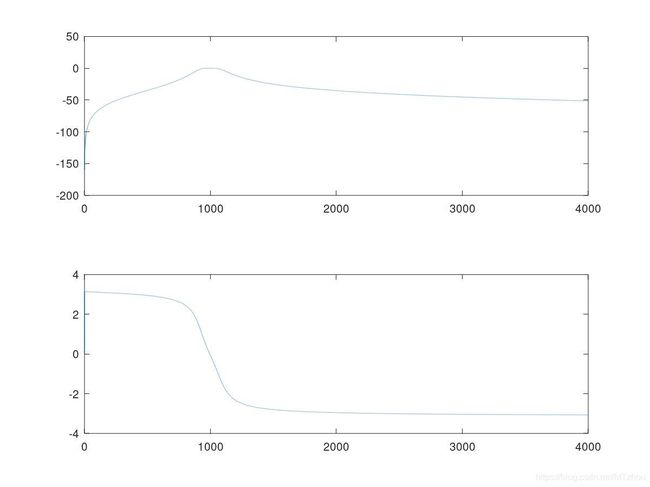
plot(F_PASS(1:Fs/6,1), Hf_PASS(1:Fs/6,1));

% Plot Phase VS Frequency
subplot(2, 1, 2);
plot(F_PASS(1:Fs/6,1), Hx_PASS(1:Fs/6,1));

plot

Stop

code

% Loader Octave packages
pkg load signal

% Sample Rate
Fs = 48000;

% Corner Frequency
F0 = 1000;
Wn = [(F0-100)/(Fs/2), (F0+100)/(Fs/2)];

[B_STOP, A_STOP] = butter(2, Wn, 'stop');
% Generate response matrix that size is Fs.
[H_STOP, w_STOP] = freqz(B_STOP, A_STOP, Fs);

% Transfer from Rad to Hz.
F_STOP = (w_STOP / (2 * pi)) * Fs;

% Transfer from Magnitude to DB
Hf_STOP = mag2db(abs(H_STOP));
Hx_STOP = angle(H_STOP);

clear figure
clf;
figure(1);

% Plot Magnitude VS Frequency
% Range: 1 ~ (Fs / 6) / 2 = 1 ~ 4000
% Because Freqz only return half result (1, +pi) rather than (-pi, +pi),
% So divided by 2.
subplot(2, 1, 1);
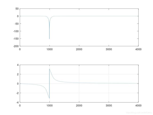
plot(F_STOP(1:Fs/6,1), Hf_STOP(1:Fs/6,1));

% Plot Phase VS Frequency
subplot(2, 1, 2);
plot(F_STOP(1:Fs/6,1), Hx_STOP(1:Fs/6,1));

plot