OpenCV官方教程中文版（For Python）

cv2.waitKey() 是一个键盘绑定函数。需要指出的是它的时间尺度是毫
秒级。函数等待特定的几毫秒，看是否有键盘输入。特定的几毫秒之内，如果 按下任意键，这个函数会返回按键的 ASCII
码值，程序将会继续运行。如果没 有键盘输入，返回值为 -1，如果我们设置这个函数的参数为 0，那它将会无限
期的等待键盘输入。它也可以被用来检测特定键是否被按下。

cv2.imwrite('messigray.png',img) 保存图像

5.2 从文件中播放视频

cv2.VideoWriter([filename, fourcc, fps, frameSize[, isColor] ])

fourcc – 4-character code of codec used to compress the frames. For example,
CV_FOURCC(’P’,’I’,’M’,’1’) is a MPEG-1 codec, CV_FOURCC(’M’,’J’,’P’,’G’) is
a motion-jpeg codec etc. List of codes can be obtained at Video Codecs by FOURCC page

10.3 按位运算
threshold：固定阈值二值化，
ret, dst = cv2.threshold(src, thresh, maxval, type)
src： 输入图，只能输入单通道图像，通常来说为灰度图
dst： 输出图
thresh： 阈值
maxval： 当像素值超过了阈值（或者小于阈值，根据type来决定），所赋予的值
type：二值化操作的类型，包含以下5种类型： cv2.THRESH_BINARY； cv2.THRESH_BINARY_INV； cv2.THRESH_TRUNC； cv2.THRESH_TOZERO；cv2.THRESH_TOZERO_INV

原文：https://blog.csdn.net/sinat_21258931/article/details/61418681
掩膜（mask）
利用掩膜（mask）进行“与”操作，即掩膜图像白色区域是对需要处理图像像素的保留，黑色区域是对需要处理图像像素的剔除，其余按位操作原理类似只是效果不同而已。
白色是255，黑色是0
这个程序原书中有一些错误，mask两个反了，然后cv2.threshold参数需要改小，不然出现的效果不对

import cv2
import numpy as np
# 加载图像
img1 = cv2.imread('C:/Users/AEC/Desktop/d.png')
img2 = cv2.imread('C:/Users/AEC/Desktop/logo.png')
# I want to put logo on top-left corner, So I create a ROI
cv2.imshow('star',img1)
cv2.imshow('logo',img2)

rows,cols,channels = img2.shape
print(rows,cols,channels)
roi = img1[0:rows, 0:cols ]
cv2.imshow('roi',roi)
# Now create a mask of logo and create its inverse mask also
img2gray = cv2.cvtColor(img2,cv2.COLOR_BGR2GRAY)
ret, mask = cv2.threshold(img2gray,25, 255, cv2.THRESH_BINARY)
cv2.imshow('mask',mask)
mask_inv = cv2.bitwise_not(mask)
cv2.imshow('mask_inv',mask_inv)
# Now black-out the area of logo in ROI
# 取 roi 中与 mask 中不为零的值对应的像素的值，其他值为 0
# 注意这里必须有 mask=mask 或者 mask=mask_inv, 其中的 mask= 不能忽略
img1_bg = cv2.bitwise_and(roi,roi,mask = mask_inv)
cv2.imshow('img1_bg',img1_bg)
# 取 roi 中与 mask_inv 中不为零的值对应的像素的值，其他值为 0。
# Take only region of logo from logo image.
img2_fg = cv2.bitwise_and(img2,img2,mask = mask)
cv2.imshow('img2_fg',img2_fg)
# Put logo in ROI and modify the main image
dst = cv2.add(img1_bg,img2_fg)
cv2.imshow('dst',dst)
img1[0:rows, 0:cols ] = dst
cv2.imshow('res',img1)
cv2.waitKey(0)
cv2.destroyAllWindows()

13.2 物体跟踪
cv2.inRange函数设阈值，去除背景部分
mask = cv2.inRange(hsv, lower_red, upper_red) #lower20===>0,upper200==>0,
函数很简单，参数有三个
第一个参数：hsv指的是原图

第二个参数：lower_red指的是图像中低于这个lower_red的值，图像值变为0

第三个参数：upper_red指的是图像中高于这个upper_red的值，图像值变为0

而在lower_red～upper_red之间的值变成255

lower_red = np.array([20, 20, 20])
upper_red = np.array([200, 200, 200])
mask = cv2.inRange(hsv, lower_red, upper_red) #lower20===>0,upper200==>0，lower～upper==>255
就是将低于lower_red和高于upper_red的部分分别变成0，lower_red～upper_red之间的值变成255
原文：https://blog.csdn.net/hjxu2016/article/details/77834599

这里一定需要注意的的问题是 这是hsv格式的图片

色调H
用角度度量，取值范围为0°～360°，从红色开始按逆时针方向计算，红色为0°，绿色为120°,蓝色为240°。它们的补色是：黄色为60°，青色为180°,品红为300°；
饱和度S
饱和度S表示颜色接近光谱色的程度。一种颜色，可以看成是某种光谱色与白色混合的结果。其中光谱色所占的比例愈大，颜色接近光谱色的程度就愈高，颜色的饱和度也就愈高。饱和度高，颜色则深而艳。光谱色的白光成分为0，饱和度达到最高。通常取值范围为0%～100%，值越大，颜色越饱和。
明度V
明度表示颜色明亮的程度，对于光源色，明度值与发光体的光亮度有关；对于物体色，此值和物体的透射比或反射比有关。通常取值范围为0%（黑）到100%（白）。

import cv2
import numpy as np
cap=cv2.VideoCapture('C:/Users/AEC/Desktop/VIDEO0077.mkv')
img = cv2.imread('C:/Users/AEC/Desktop/1550668243(1).png')
print(img)
print(img.shape)
while(1):
    # 获取每一帧
    ret,frame=cap.read()
    # 转换到 HSV
    hsv=cv2.cvtColor(frame,cv2.COLOR_BGR2HSV)
    # 设定红色的阈值
    lower_red=np.array([160,0,0])
    upper_red=np.array([360,255,255])
    # 根据阈值构建掩模
    mask=cv2.inRange(hsv,lower_blue,upper_blue)
    # 对原图像和掩模进行位运算
    res=cv2.bitwise_and(frame,frame,mask=mask)
    # 显示图像
    cv2.imshow('frame',frame)
    cv2.imshow('mask',mask)
    cv2.imshow('res',res)
    k=cv2.waitKey(100)&0xFF
    if k==27:
        break
# 关闭窗口
cv2.destroyAllWindows()

用保温杯测试的识别效果

不得不说掩模运算这个东西真的好神奇啊！
13.3 找到跟踪对象的HSV值

函数 cv2.cvtColor() 也可以用到这里。但是现在你要传入的参数是（你想要 的）BGR 值而不是一副图。例如，我们要找到绿色的
HSV 值，我们只需在终 端输入以下命令：

# -*- coding: utf-8 -*-
"""
Created on Fri Jan 10 20:34:29 2014
@author: duan
"""
import cv2
import numpy as np
green=np.uint8([0,255,0])
hsv_green=cv2.cvtColor(green,cv2.COLOR_BGR2HSV)
error: /builddir/build/BUILD/opencv-2.4.6.1/
modules/imgproc/src/color.cpp:3541:
error: (-215) (scn == 3 || scn == 4) && (depth == CV_8U || depth == CV_32F)
in function cvtColor
#scn (the number of channels of the source),
#i.e. self.img.channels(), is neither 3 nor 4.
#
#depth (of the source),
#i.e. self.img.depth(), is neither CV_8U nor CV_32F.
# 所以不能用 [0,255,0]，而要用 [[[0,255,0]]]
# 这里的三层括号应该分别对应于 cvArray，cvMat，IplImage
green=np.uint8([[[0,255,0]]])
hsv_green=cv2.cvtColor(green,cv2.COLOR_BGR2HSV)
print hsv_green
[[[60 255 255]]]
现在你可以分别用 [H-100，100，100] 和 [H+100，255，255] 做上
下阈值。除了这个方法之外，你可以使用任何其他图像编辑软件（例如 GIMP）
或者在线转换软件找到相应的 HSV 值，但是最后别忘了调节 HSV 的范围。

14 几何变换
缩放 cv2.resize(src, dsize[, dst[, fx[, fy[, interpolation ] ] ] ]) → dst
平移 cv2.warpAffine()
旋转 cv2.getRotationMatrix2D
仿射变换 cv2.getAffineTransform + cv2.warpAffine
透视变换 cv2.getPerspectiveTransform() +cv2.warpAffine

15 图像阈值

阈值分割处理主要是根据灰度值信息提取前景，所以对前景物体与背景有较强对比度的图像的分割特别有用。对对比度很弱的图像进行阈值分割，需要先进行图像的对比度增强，然后再进行阈值处理。下面介绍两种常用的阈值分割技术：全局阈值分割和自适应局部阈值分割

• 全局阈值分割

1 Ostu算法 前景与背景灰度平均值差距大 处理效果比2，3更好
2 熵算法 自动计算阈值 不满足双峰图像也适用
3直方图技术法 前景与背景对比明显的图像包含双峰 处理效果较好

• 局部阈值分割 （如受光照不均变化影响）

1自适应阈值算法 不均匀照明或者灰度分布不均效果好

1 ostu二值化 算法原理

我写了一个python程序，实现这个算法

from matplotlib import pyplot as plt
import numpy as np
import cv2
import math

img = cv2.imread('C:/Users/AEC/Desktop/2.png',0)
#灰度值数组
global calhist
calhist = cv2.calcHist([img],[0],None,[256],[0,256])
#灰度值总和
global N
N = np.sum(calhist)

#绘制灰度直方图
plt.hist(img.ravel(),256,[0,256])
plt.show()

#返回k的零阶累计矩
def zeroCumuMoment(k):
    sum0 = 0
    for i in range (0,k+1):#注意左闭右开，故k需要+1
        sum0 = sum0 + calhist[i]/N
    return sum0
    
#返回k的一阶累计矩
def OneCumuMoment(k):
    sum1 = 0
    for i in range(0,k+1):
        sum1 = sum1 + calhist[i]/N * i
    return sum1
    
#图像总体灰度平均值
global mean
mean = OneCumuMoment(255)

#计算不同k值下方差大小
def choosek(k):
    u0 = OneCumuMoment(k) / (zeroCumuMoment(k))#前景区域平均灰度
    u1 = (mean - OneCumuMoment(k)) / (1 - zeroCumuMoment(k))#背景区域平均灰度
    fangcha = math.pow((u0 - mean), 2) * zeroCumuMoment(k) + math.pow((u1 - mean), 2) * (1 - zeroCumuMoment(k))
    return fangcha
    
#选出方差最大的k值即为像素阈值
fangcha = []
for i in range(0,256):
    fangcha.append(choosek(i))
print(np.argmax(fangcha))

#采用cv2的包计算出的像素阈值
ret2,th2 = cv2.threshold(img,0,255,cv2.THRESH_BINARY+cv2.THRESH_OTSU)
print(ret2)

经过检验，程序得到的阈值和cv2包中计算的阈值相等
2 熵算法

图像可以看成一种信源，算法步骤

基于以上算法，我写的计算熵值的程序

import cv2
import numpy as np
import math
from matplotlib import pyplot as plt

img = cv2.imread('C:/Users/AEC/Desktop/3.png',0)
rows,cols = img.shape
#灰度值数组
global calhist
calhist = cv2.calcHist([img],[0],None,[256],[0,256])
#灰度值总和
global N
N = np.sum(calhist)
#归一化灰度值数组
calhist = calhist / N
#绘制灰度直方图
plt.subplot(212)#分成2*1，占用第二个
plt.hist(img.ravel(),256,[0,256]),plt.title('hist')

#返回k的零阶累计矩
def zeroCumuMoment(k):
    sum0 = 0
    for i in range (0,k+1):#注意左闭右开，故k需要+1
        sum0 = sum0 + calhist[i]
    return sum0

def calHB(k):
    #背景累积概率
    zerocumumomentb = zeroCumuMoment(k)
    #背景熵
    hb = 0
    for i in range(0,k+1):
        if zerocumumomentb == 0:
            i = i+1
            continue
            pb = calhist[i] / zerocumumomentb
            if pb == 0:
                i = i+1
                continue
            hb = hb - (pb * math.log(pb))
    return hb

def calHF(k):
    #前景累积概率
    zerocumumomentf = 1-zeroCumuMoment(k)
    #前景熵
    hf = 0
    for i in range(k+1,256):
        pf = calhist[i] / zerocumumomentf
        if pf == 0:
            i = i+1
            continue
        hf = hf - (pf * math.log(pf))
    return hf

entropy = []
for i in range(0,256):
    h = calHB(i) + calHF(i)
    entropy.append(h)

threshold = np.argmax(entropy)
print('entropythreshold = ' + str(threshold))
#作图
plt.subplot(221)#分成2*2，占用第一个
plt.imshow(img),plt.title('origin pic')
ret1,th1 = cv2.threshold(img,threshold,255,cv2.THRESH_BINARY)
plt.subplot(222)#分成2*2，占用第二个
plt.imshow(th1),plt.title('entropy pic')
plt.show()
cv2.waitKey(0)

结果图：可以看出分割结果较好
ps 这里我计算的阈值是100，但书上是62，对比了一下62和100时的分割效果，觉得书上应该不对，或者是图片的关系，我没有原图，所以直接用的截图来做的。

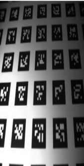
自适应阈值 针对光照不均匀情况
可以采用均值平滑，高斯平滑，中值平滑三种平滑处理方式，这三种平滑处理方法对自适应阈值分割的结果还是有一些区别的，所以在处理特定问题时，需要通过实验对比的方式，选择其中一种比较理想的平滑方式。
这是原图，可以看出光照不均匀

import cv2
import numpy as np
from matplotlib import pyplot as plt

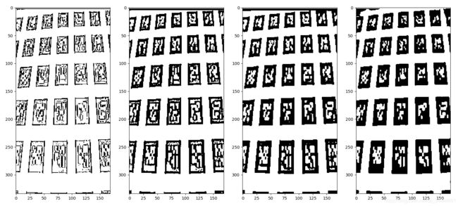
img = cv2.imread('C:/Users/AEC/Desktop/4.png')
def adaptiveThreshold(img,winsize,ratio):
    #平滑处理
    img_mean = cv2.boxFilter(img,cv2.CV_32FC1,winsize)
    #自适应阈值矩阵
    Thresh = img-(1-ratio)*img_mean
    Thresh[Thresh>=0] = 255
    Thresh[Thresh<0] = 0
    Thresh =  Thresh.astype(np.uint8)
    return  Thresh

imgs = []
#不同大小的均值平滑算子
winsizes = [(3,3),(7,7),(11,11),(31,31)]
i = 1
for winsize in winsizes:
    print(winsize)
    imgs.append(adaptiveThreshold(img,winsize,0.15))
    plt.subplot(1,4,i)
    plt.imshow(imgs[i-1])
    i = i+1
plt.show()

当平滑算子较大时效果比较理想

16 图像平滑

常用的平滑处理算法包括基于二维离散卷积的高斯平滑、均值平滑，基于统计学方法的中值平滑，具备保持边缘作用的平滑算法的双边滤波、导向滤波等

• 低通滤波去除噪音，模糊图像
• 高通滤波找到图像边缘

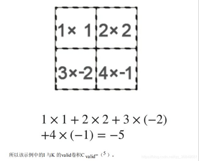
1 二维离散卷积 二维离散卷积是基于两个矩阵的计算形式，

• Full卷积

1 将K逆时针转180°得到Kflip
2 Kflip沿着I按照先行后列的顺序，每移动到一个固定位置，对应位置就相乘，然后求和。
例子：

• valid卷积 只是考虑I 能完全覆盖K f lip内的值的情况，该过程称为valid卷积
  
• same卷积 中给K f lip指定一个“锚点”，然后将“锚点”循环移至图像矩阵的（r，c）处
  
• convolved2d(in1,in2,mode=‘full’,boundary=‘fill’,fillvalue=0)

图像模糊的四个方法

• 1 平均 归一化卷积，卷积框覆盖区域所有像素的平均值代替中心元素
  cv2.blur()或者cv2.boxFilter()
• 2 高斯模糊 卷积框里的值符合高斯分布
  cv2.GaussianBlur()
  -3 中值模糊 用与卷积框对应的像素的中值替代中心像素的值 用于去除椒盐噪声
  cv2.medianBlur()
  -4 双边滤波 保持边界清晰的情况下有效去除噪声
  cv2.bilateralFilter()

同时使用空间高斯权重和灰度值相似性高斯权重
空间高斯函数确保只有邻近区域的像素对中心点有影响，灰度值相似性高斯函数确保只有与中心像素灰度值相近的才会被用来做模糊运算。所以这种方法会确保边界不会被模糊掉，因为边界处的灰度值变化比较大

2 高斯模糊


高斯模糊平滑图像的原理我的理解是：高斯模糊实际是做了个加权平均，因此变化剧烈的高频成分，如边缘、条纹、噪点等像素将会变得平滑（即被“压抑”）。而原本比较平滑的地方，做了加权平均一样比较平滑，变化不大（即被“通过”）。σ越小，曲线越尖，高斯核的中心像素的权重也就越大，周围的权重就越小，模糊程度也就越弱。反之，σ越大，则模糊程度越重。

17 形态学转换
17.1 腐蚀 取每个位置的邻域内值的最小值作为该位置的输出灰度值，邻域结构形状是结构元：椭圆形、矩形、十字交叉形
cv2.erode(src, kernel[, dst[, anchor[, iterations[, borderType[, borderValue ] ] ] ] ]) → dst
17.2 膨胀 取最大值，较亮物体尺寸增大，较暗物体尺寸减小
Python: cv2.dilate(src, kernel[, dst[, anchor[, iterations[, borderType[, borderValue ] ] ] ] ]) → dst
17.3 开运算 先腐蚀后膨胀 消除暗背景下的亮点

17.4 闭运算 先膨胀后腐蚀 填充白色物体里的黑色空洞

17.5 形态学梯度 膨胀结果-腐蚀结果 得到边界
gradient = cv2.morphologyEx(img, cv2.MORPH_GRADIENT, kernel)
17.6 白顶帽运算 图像-开运算
tophat = cv2.morphologyEx(img, cv2.MORPH_TOPHAT, kernel)
17.7 黑底帽运算 图像-闭运算
blackhat = cv2.morphologyEx(img, cv2.MORPH_BLACKHAT, kernel)
结构化元素
cv2.getStructuringElement(cv2.MORPH_RECT,(5,5))
构建不同形状的核

Roberts算子/Prewitt边缘检测 差分

18.1 sobel算子 高斯平滑+差分
python实现

import numpy as np
import cv2
import math
from scipy import signal
from matplotlib import pyplot as plt
#窗口大小为n的高斯平滑算子
def gausssmooth(n):
    gaussmooths = np.zeros([1,n],np.float32)
    for r in range(n):
        #二项式系数
        gaussmooth = math.factorial(n-1)/(math.factorial(r)*math.factorial(n-r-1))
        gaussmooths[0][r] = gaussmooth

    return gaussmooths

    #差分算子
def differential(n):
    if n == 1:
        differentials = np.array([1,-1],np.float32)
    elif n == 2:
        differentials = np.array([1, 0,-1], np.float32)
    elif n == 3:
        differentials = np.array([1, 1,-1, -1], np.float32)
    else:
        differentials = np.zeros([1,n+1],np.float32)
        differentials[0][0]=0
        differentials[0][n]=0
        for r in range(0,n-1):
            # 二项式系数
            differential = math.factorial(n - 2) / (math.factorial(r) * math.factorial(n - r - 2))
            differentials[0][r+1] = differential
        newdifferentials = np.zeros([1,n])
        for i in reversed(range(1,n+1)):
            newdifferentials[0][i-1] = differentials[0][i]-differentials[0][i-1]
    return newdifferentials


#灰度图
img = cv2.imread('C:/Users/AEC/Desktop/1.png',cv2.IMREAD_GRAYSCALE)
#设置sobel算子
n=5
sobel_x = signal.convolve2d(gausssmooth(n).transpose(), differential(n), mode='full')
sobel_y = signal.convolve2d(gausssmooth(n), differential(n).transpose(), mode='full')

img_sobel_x = signal.convolve2d(img, sobel_x, mode='same')
img_sobel_y = signal.convolve2d(img, sobel_y, mode='same')

#总体边缘并归一化
edge = np.sqrt(np.power(img_sobel_x,2.0)+np.power(img_sobel_y,2.0))
edge1 = edge/np.max(edge)
edge1 = edge1 * 255
edge1 = edge1.astype(np.uint8)
#x边缘，绝对值处理，归一化
edge_x = np.abs(img_sobel_x)/np.max(img_sobel_x)
edge_x = edge_x * 255
edge_x = edge_x.astype(np.uint8)
#y边缘，绝对值处理，归一化
edge_y = np.abs(img_sobel_y)/np.max(img_sobel_y)
edge_y = edge_y * 255
edge_y = edge_y.astype(np.uint8)

plt.subplot(221),plt.imshow(img),plt.title('the origin')
plt.subplot(222),plt.imshow(edge),plt.title('edge')
plt.subplot(223),plt.imshow(edge_x),plt.title('edge_x')
plt.subplot(224),plt.imshow(edge_y),plt.title('edge_y')
plt.show()
cv2.waitKey()

效果图

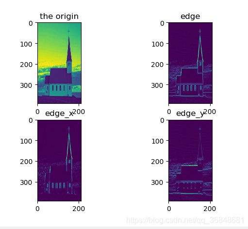
使用高阶sobel算子得到的边缘信息会比低阶丰富

cv.Sobel(src, dst, xorder, yorder, apertureSize=3) → None
Parameters
src – input image.
dst – output image of the same size and the same number of channels as src .
ddepth –
output image depth; the following combinations of src.depth() and ddepth are supported:
– src.depth() = CV_8U, ddepth = -1/CV_16S/CV_32F/CV_64F
– src.depth() = CV_16U/CV_16S, ddepth = -1/CV_32F/CV_64F
– src.depth() = CV_32F, ddepth = -1/CV_32F/CV_64F
– src.depth() = CV_64F, ddepth = -1/CV_64F
when ddepth=-1, the destination image will have the same depth as the source; in the case
of 8-bit input images it will result in truncated derivatives.
xorder – order of the derivative x.
yorder – order of the derivative y.
ksize – size of the extended Sobel kernel; it must be 1, 3, 5, or 7.

Kirsch算子/Robinson算子
都是八个卷积核，然后图像与每个核分别进行卷积，取对应位置绝对值最大的值作为最后输出的边缘强度
由于使用了八个方向的卷积核，因此检测到的边缘比标准的Prewitt算子和sobel算子检测到的边缘会显得更加丰富。

这个函数写的还是很厉害的，主要（edge>=list_edge[i])它本身其实就可以看成对每个元素的遍历

注意取绝对值以及分别阈值处
sobel_x = signal.convolve2d(gausssmooth(n).transpose(), differential(n), mode='full')
sobel_y = signal.convolve2d(gausssmooth(n), differential(n).transpose(), mode='full')

img_sobel_x = np.abs(signal.convolve2d(img, sobel_x, mode='same'))
img_sobel_x[img_sobel_x>255]=255
img_sobel_y = np.abs(signal.convolve2d(img, sobel_y, mode='same'))
img_sobel_y[img_sobel_y>255]=255
#总体边缘并归一化
edge = np.sqrt(np.power(img_sobel_x,2.0)+np.power(img_sobel_y,2.0))
edge[edge>255]=255
edge = edge.astype(np.uint8)

canny算子
如果我用python写出来了我就应该也蛮佩服我自己的了
写出来了虽然写了很久然后两个低级BUG导致我一直怀疑显卡不够，双阈值的连结性那块还是看了源程序，这种递归感觉的不太会写。

顺一下思路
首先canny算子是对sobel、prewitt算法的改进，sobel算法没有充分利用边缘的梯度方向这一条件，并且在最后输出的边缘二值图中，只是简单地利用阈值进行处理，如果阈值过大，则会损失很多边缘信息，而阈值过小则会有很多噪声，因此canny边缘检测基于这两点进行了改进：
1 利用边缘梯度方向进行非极大值抑制
2 利用双阈值以及连接性进行滞后阈值处理

第一步：进行sobel运算，得到卷积核sobel_x,sobel_y,并将img分别与两个卷积核进行卷积得到img_sobel_x,img_sobel_y
然后进行开方就可以得到边缘强度magnitude
从图像的角度考虑，这一步就是提取边缘 用赫敏的图写程序会开心一点o(￣▽￣)ブ

第二步： 进行插值运算
非极大值抑制，只保留了极大值，抑制了非极大值，所以该步骤实际上是对Sobel边缘的细化，每个边缘只保留最明显的一个像素点就可以，也就是保留极大值。

第三步 双阈值的滞后阈值处理
1 边缘强度大于高阈值，作为确定边缘点
2 边缘强度低于阈值点剔除
3 边缘强度在中间的，只有这些点能够按照某一路径与确定边缘点相连时，才可以作为边缘点被接受，组成这一路径的所有点的边缘强度都比低阈值大
这个程序跑不通，因为说显卡内存不够？？？？？
跑通了。。有两个很低级的BUG
1 记得写range(1,n)不然出来像素点值全是0
2 比较复杂的公式括号要打对

import numpy as np
import cv2
import math
import sobelcal
from matplotlib import pyplot as plt

#非极大值抑制
def non_maximum_suppression_Inter(dx,dy):
    rows, cols = dx.shape
    edgeMag_nonMaxSup = np.zeros(dx.shape)
    for r in range(1,rows-1):
        for c in range(1,cols-1):
            if dx[r][c]==0 or dy[r][c]==0 :
                continue
            angle = math.atan2(dy[r][c],dx[r][c])/math.pi*180
            if(angle>45 and angle<=90) or (angle>-135 and angle <=-90):
                chazhi1 = dx[r][c]/dy[r][c]*magnitude[r-1][c-1]+(1-dx[r][c]/dy[r][c])*magnitude[r-1][c]
                chazhi2 = dx[r][c]/dy[r][c]*magnitude[r+1][c+1]+(1-dx[r][c]/dy[r][c])*magnitude[r+1][c]
                if (magnitude[r][c]>chazhi1 and magnitude[r][c]>chazhi2):
                    edgeMag_nonMaxSup[r][c] = magnitude[r][c]
            if (angle> 90 and angle<= 135) or (angle> -90 and angle <= -45):
                chazhi1 = np.abs(dx[r][c]/dy[r][c])*magnitude[r-1][c+1] + (1-np.abs(dx[r][c]/dy[r][c]))*magnitude[r-1][c]
                chazhi2 = np.abs(dx[r][c]/dy[r][c])*magnitude[r+1][c-1] +(1-np.abs(dx[r][c]/dy[r][c]))*magnitude[r+1][c]
                if (magnitude[r][c] > chazhi1 and magnitude[r][c] > chazhi2):
                    edgeMag_nonMaxSup[r][c] = magnitude[r][c]
            if (angle >= 0 and angle <= 45) or (angle >= -180 and angle <= -135):
                chazhi1 = (dy[r][c]/dx[r][c])*magnitude[r-1][c-1]+(1-(dy[r][c]/dx[r][c]))*magnitude[r][c-1]
                chazhi2 = (dy[r][c]/dx[r][c])*magnitude[r+1][c+1]+(1-(dy[r][c]/dx[r][c]))*magnitude[r][c+1]
                if (magnitude[r][c] > chazhi1) and (magnitude[r][c] > chazhi2):
                    edgeMag_nonMaxSup[r][c] = magnitude[r][c]
            if (angle > 135 and angle <= 180) or (angle > -45 and angle < 0):
                chazhi1 = np.abs(dy[r][c]/dx[r][c])*magnitude[r-1][c+1]+(1-np.abs(dy[r][c]/dx[r][c]))*magnitude[r][c+1]
                chazhi2 = np.abs(dy[r][c]/dx[r][c])*magnitude[r+1][c-1]+(1-np.abs(dy[r][c]/dx[r][c]))*magnitude[r][c-1]
                if (magnitude[r][c] > chazhi1) and (magnitude[r][c] > chazhi2):
                    edgeMag_nonMaxSup[r][c] = magnitude[r][c]
    return edgeMag_nonMaxSup

def checkinRange(r,c,rows,cols):
    if r>=0 and r=0 and c= lowerThresh:
                    trace(maximum_suppression, edge, lowerThresh, r + i, c + j, rows, cols)
#这一步是检查强像素点八个领域的点，如果既在图像上，值又大于最低阈值，那么就保留他，并顺着她找下一个点

#双阈值滞后
def hysteresisThreshold(maximum_suppression,lowerThresh,upperThresh_):
    rows,cols = maximum_suppression.shape
    edge = np.zeros(maximum_suppression.shape,np.uint8)
    for r in range(1,rows-1):
        for c in range(1,cols-1):
            if maximum_suppression[r][c]>=upperThresh_:
                trace(maximum_suppression,edge,lowerThresh,r,c,rows,cols)
            if maximum_suppression[r][c]255]=255
magnitude = magnitude.astype(np.uint8)
plt.subplot(131),plt.imshow(magnitude,cmap='gray'),plt.title('magnitude')

#边缘强度非极大值抑制
maximum_suppression = non_maximum_suppression_Inter(image_sobel_x,image_sobel_y)
maximum_suppression[maximum_suppression>255]=255
maximum_suppression=maximum_suppression.astype(np.uint8)
plt.subplot(132),plt.imshow(maximum_suppression,cmap='gray'),plt.title('maximum_suppression')

#双阈值滞后阈值处理
edge = hysteresisThreshold(maximum_suppression,60,100)
plt.subplot(133),plt.imshow(edge,cmap='gray'),plt.title('canny')
#plt显示灰度图
plt.show()
cv2.destroyAllWindows()

1 拉普拉斯算子

常见形式

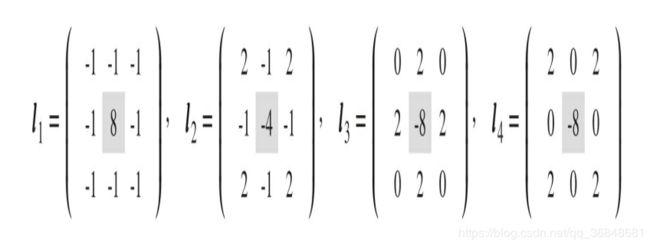
2 拉普拉斯算子对噪声很敏感 ，因此先对图像高斯平滑，再与拉普拉斯算子卷积，最后0阈值化
LOG 高斯拉普拉斯边缘检测
构建LOG卷积核，通过一次卷积就可以得到边缘

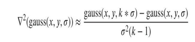
3 DOG高斯差分边缘检测
k=0.95时 高斯拉普拉斯和高斯差分近似相等，先计算差分算子，然后零阈值处理

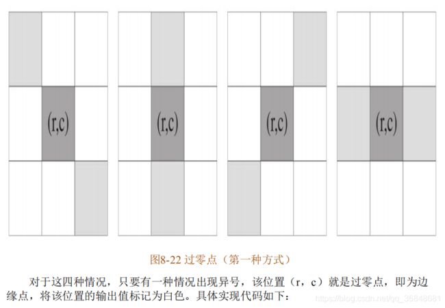
4 Marr-Hildreth 边缘检测
对高斯差分和高斯拉普拉斯检测到的边缘的细化 ，卷积后结果寻找二阶导为0(过零点)的位置即为边缘位置
二阶导为0即变化率最大的位置，可以获得封闭边缘

霍夫检测！
整理下思路
1首先把图片，灰度化，canny算子找到边缘，得到一个二值化图像，前景像素用白色（灰度值255），背景色用黑色（灰度值0）
2 检验哪些白色像素点共线，根据每个白色像素点的坐标，离散化，每隔1°计算一个对应的角度，每隔1计算一个幅值，我的感觉是把直角坐标系转到极坐标系，然后极坐标每隔一个角度算一次，最后进行投票，记录下投票数高的点的坐标，然后cv2.line画线就行
霍夫检测书上的源码又出现了一个问题，我感觉是因为他的x,y坐标计算的时候的坐标系和正常图像的坐标点是反的，导致如果按照他那样写，刚好检测到的线是对称反着的。

import sys
import numpy as np
import cv2
import math
from matplotlib import pyplot as plt
from mpl_toolkits.mplot3d import Axes3D
def HTline(img,steptheta,steprho):
    #宽、高
    rows,cols = img.shape
    #图像中可能出现的最大长度
    L = round(math.sqrt(pow(rows,2.0)+pow(cols,2.0)))+1
    numtheta = int(180.0/steptheta)
    numrho = int(2*L/steprho)+1
    accumulator = np.zeros((numrho,numtheta),np.int32)
    #建立字典，存储点坐标
    accuDict = {}
    for k1 in range(-L,L+1,steprho):
        for k2 in range(numtheta):
            accuDict[(k1,k2)]=[]
    #投票计数
    for y in range(rows):
        for x in range(cols):
            if img[y][x]==255:
                for m in range(numtheta):
                    rho =round(x*math.cos(steptheta*m/180.0*math.pi)+y*math.sin(steptheta*m/180.0*math.pi))
                    accumulator[rho,m]+=1
                    accuDict[(rho,m)].append((x,y))#这里xy坐标得换过来
    return accuDict,accumulator
    
# 主函数
if __name__=='__main__':
    img = cv2.imread('C:/Users/AEC/Desktop/img2.jpg',0)
    #canny 边缘检测
    edge = cv2.Canny(img,50,200)
    #显示二值化边缘
    cv2.imshow('edge',edge)
    #霍夫直线检测
    accuDict,accumulator = HTline(edge,1,1)
    #计数器三维显示
    rows,cols = accumulator.shape
    fig = plt.figure()
    ax = fig.gca(projection='3d')
    X,Y = np.mgrid[0:rows:1,0:cols:1]
    surf = ax.plot_wireframe(X,Y,accumulator,cstride=1,rstride=1,color='gray')
    ax.set_xlabel(u"$\\rho$")
    ax.set_ylabel(u"$\\theta$")
    ax.set_zlabel("accumulator")
    ax.set_zlim3d(0,np.max(accumulator))
    # 只画出投票数大于60的直线
    voteThresh = 60
    for r in range(rows):
        for c in range(cols):
            if accumulator[r][c]>voteThresh:
                points = accuDict[(r,c)]
                print(points)
                cv2.line(img,points[0],points[len(points)-1],(255),2)#画线
    cv2.imshow("I",img)
    plt.show()
    cv2.waitKey(0)

霍夫检测效果图