计算机视觉第三次实验——SIFT特征提取与检索
文章目录
- 计算机视觉第三次实验——SIFT特征提取与检索
- 一,安装VLfeat
- 1.1 下载地址
- 1.2 注意
- 二,获取像素集
- 三,描述子代码了实现
- 3.1 代码
- 3.2 结果
- 四,匹配描述子代码实现
- 4.1代码
- 4.2 结果
- 五,给定一张输入的图片,在数据集内部进行检索,输出与其匹配最多的三张图片
- 5.1代码
- 5.2 结果
- 六,匹配地理标记图像
- 6.1代码实现
- 6.2代码结果
- 6.3 结果分析
- 6.4错误分析
- 七,RANSAC算法
- 7.1概况
- ransac
- 7.2算法步骤
- 7.3代码
- 7.4实验结果
- 7.5实验小结:
- 八实验小结
- 8.1 实验过程中的错误以及解决方法
- 8.2 SIFT的缺点
- 8.3 对比Harris算子
计算机视觉第三次实验——SIFT特征提取与检索
一,安装VLfeat
1.1 下载地址
首先,在使用SIFT算法的时候,我们需要用到python的第三方库VLfeat。其中包含了SIFT算法以及其他的函数方法。下载链接: http://www.vlfeat.org/download/
1.2 注意
这里应该下载0.9.20版本的才可用,我下载的是vIfeat-0.9.20-bin.tar.gz。下载完后解压)
接下来需要进行的操作步骤:
1、把vIfeat文件夹 下win64中的sift.exe和v.dI这两个文件复制到项目的文件夹中。
2、修改Anaconda文件夹下的PCV (我的PCV位置E:\Anaconda\Anaconda3\Lib\site-packages\PCV)文件夹里面的localdescriptors文件夹中的sift.py文件,使用记事本打开,修改其中的cmmd内的路径为: cmmd =str(r"D:\PythonWork\SIFT\sift.exe “+ imagename+”–output=” + resultname+" "+params) (路径是你项目文件夹中的ift.exe的路径)然后要记得在括号内加r! !不然会出错! !
然后就能够运行了。如果在运行过程中提示关于print的错误,记得根据错误提醒的文件夹,去修改相应的print语法, 3.5的python的print用法是需要加括号。
二,获取像素集

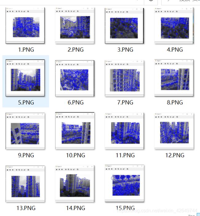
三,描述子代码了实现
3.1 代码
# -*- coding: utf-8 -*-
from PIL import Image
from pylab import *
from numpy import *
import os

def process_image(imagename, resultname, params="--edge-thresh 10 --peak-thresh 5"):
    """ 处理一幅图像,然后将结果保存在文件中"""

    if imagename[-3:] != 'pgm':
        #创建一个pgm文件
        im = Image.open(imagename).convert('L')
        im.save('tmp.pgm')
        imagename ='tmp.pgm'
    cmmd = str("sift "+imagename+" --output="+resultname+" "+params)
    os.system(cmmd)
    print 'processed', imagename, 'to', resultname

def read_features_from_file(filename):
    """读取特征属性值,然后将其以矩阵的形式返回"""
    f = loadtxt(filename)
    return f[:,:4], f[:,4:] #特征位置,描述子

def write_featrues_to_file(filename, locs, desc):
    """将特征位置和描述子保存到文件中"""
    savetxt(filename, hstack((locs,desc)))

def plot_features(im, locs, circle=False):
    """显示带有特征的图像
       输入:im(数组图像),locs(每个特征的行、列、尺度和朝向)"""

    def draw_circle(c,r):
        t = arange(0,1.01,.01)*2*pi
        x = r*cos(t) + c[0]
        y = r*sin(t) + c[1]
        plot(x, y, 'b', linewidth=2)

    imshow(im)
    if circle:
        for p in locs:
            draw_circle(p[:2], p[2])
    else:
        plot(locs[:,0], locs[:,1], 'ob')
    axis('off')

imname = r'C:\Users\59287\PycharmProjects\untitled1\sift\15.jpg'
im1 = array(Image.open(imname).convert('L'))
process_image(imname, '15.sift')
l1,d1 = read_features_from_file('15.sift')

figure()
gray()
plot_features(im1, l1, circle=True)
show()
3.2 结果
四,匹配描述子代码实现
对于将一幅图像中的特征匹配到另一幅图像的特征,一种稳健的准则(是由 Lowe 提出的)是使用这两个特征距离和两个最匹配特征距离的比率。相比于图像 中的其他特征,该准则保证能够找到足够相似的唯一特征。使用该方法可以使错误 的匹配数降低。
4.1代码
# -*- coding: utf-8 -*-
from PIL import Image
from pylab import *
from numpy import *
import os

def process_image(imagename, resultname, params="--edge-thresh 10 --peak-thresh 5"):
    """ 处理一幅图像,然后将结果保存在文件中"""

    if imagename[-3:] != 'pgm':
        #创建一个pgm文件
        im = Image.open(imagename).convert('L')
        im.save('tmp.pgm')
        imagename ='tmp.pgm'
    cmmd = str("sift "+imagename+" --output="+resultname+" "+params)
    os.system(cmmd)
    print 'processed', imagename, 'to', resultname

def read_features_from_file(filename):
    """读取特征属性值,然后将其以矩阵的形式返回"""
    f = loadtxt(filename)
    return f[:,:4], f[:,4:] #特征位置,描述子

def write_featrues_to_file(filename, locs, desc):
    """将特征位置和描述子保存到文件中"""
    savetxt(filename, hstack((locs,desc)))

def plot_features(im, locs, circle=False):
    """显示带有特征的图像
       输入:im(数组图像),locs(每个特征的行、列、尺度和朝向)"""

    def draw_circle(c,r):
        t = arange(0,1.01,.01)*2*pi
        x = r*cos(t) + c[0]
        y = r*sin(t) + c[1]
        plot(x, y, 'b', linewidth=2)

    imshow(im)
    if circle:
        for p in locs:
            draw_circle(p[:2], p[2])
    else:
        plot(locs[:,0], locs[:,1], 'ob')
    axis('off')

def match(desc1, desc2):
    """对于第一幅图像中的每个描述子,选取其在第二幅图像中的匹配
    输入:desc1(第一幅图像中的描述子),desc2(第二幅图像中的描述子)"""
    desc1 = array([d/linalg.norm(d) for d in desc1])
    desc2 = array([d/linalg.norm(d) for d in desc2])

    dist_ratio = 0.6
    desc1_size = desc1.shape
    matchscores = zeros((desc1_size[0],1),'int')
    desc2t = desc2.T #预先计算矩阵转置
    for i in range(desc1_size[0]):
        dotprods = dot(desc1[i,:],desc2t) #向量点乘
        dotprods = 0.9999*dotprods
        # 反余弦和反排序,返回第二幅图像中特征的索引
        indx = argsort(arccos(dotprods))

        #检查最近邻的角度是否小于dist_ratio乘以第二近邻的角度
        if arccos(dotprods)[indx[0]] < dist_ratio * arccos(dotprods)[indx[1]]:
            matchscores[i] = int(indx[0])

    return matchscores

def match_twosided(desc1, desc2):
    """双向对称版本的match()"""
    matches_12 = match(desc1, desc2)
    matches_21 = match(desc2, desc1)

    ndx_12 = matches_12.nonzero()[0]

    # 去除不对称的匹配
    for n in ndx_12:
        if matches_21[int(matches_12[n])] != n:
            matches_12[n] = 0

    return matches_12

def appendimages(im1, im2):
    """返回将两幅图像并排拼接成的一幅新图像"""
    #选取具有最少行数的图像,然后填充足够的空行
    rows1 = im1.shape[0]
    rows2 = im2.shape[0]

    if rows1 < rows2:
        im1 = concatenate((im1, zeros((rows2-rows1,im1.shape[1]))),axis=0)
    elif rows1 >rows2:
        im2 = concatenate((im2, zeros((rows1-rows2,im2.shape[1]))),axis=0)
    return concatenate((im1,im2), axis=1)

def plot_matches(im1,im2,locs1,locs2,matchscores,show_below=True):
    """ 显示一幅带有连接匹配之间连线的图片
        输入:im1, im2(数组图像), locs1,locs2(特征位置),matchscores(match()的输出),
        show_below(如果图像应该显示在匹配的下方)
    """
    im3=appendimages(im1,im2)
    if show_below:
        im3=vstack((im3,im3))
    imshow(im3)

    cols1 = im1.shape[1]
    for i in range(len(matchscores)):
        if matchscores[i]>0:
            plot([locs1[i,0],locs2[matchscores[i,0],0]+cols1], [locs1[i,1],locs2[matchscores[i,0],1]],'c')
    axis('off')

# 示例
im1f = r'C:\Users\59287\PycharmProjects\untitled1\sift\9.jpg'
im2f = r'C:\Users\59287\PycharmProjects\untitled1\sift\15.jpg'
im1 = array(Image.open(im1f))
im2 = array(Image.open(im2f))

process_image(im1f, 'out_sift_1.txt')
l1,d1 = read_features_from_file('out_sift_1.txt')
figure()
gray()
subplot(121)
plot_features(im1, l1, circle=False)

process_image(im2f, 'out_sift_2.txt')
l2,d2 = read_features_from_file('out_sift_2.txt')
subplot(122)
plot_features(im2, l2, circle=False)

matches = match_twosided(d1, d2)
print '{} matches'.format(len(matches.nonzero()[0]))
figure()
gray()
plot_matches(im1,im2,l1,l2,matches, show_below=True)
show()
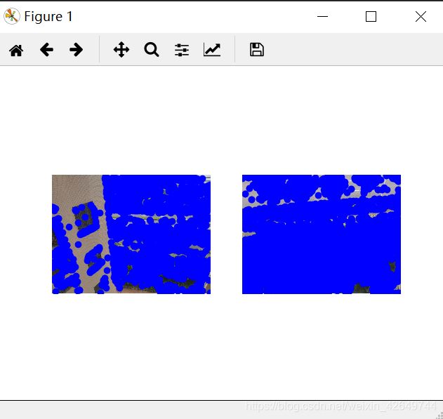
4.2 结果

五,给定一张输入的图片,在数据集内部进行检索,输出与其匹配最多的三张图片
5.1代码
# -*- coding: utf-8 -*-
from PIL import Image
from pylab import *
from numpy import *
import os
from PCV.tools.imtools import get_imlist  # 导入原书的PCV模块
import matplotlib.pyplot as plt  # plt 用于显示图片
import matplotlib.image as mpimg  # mpimg 用于读取图片


def process_image(imagename, resultname, params="--edge-thresh 10 --peak-thresh 5"):
    """ 处理一幅图像,然后将结果保存在文件中"""
    if imagename[-3:] != 'pgm':
        # 创建一个pgm文件
        im = Image.open(imagename).convert('L')
        im.save('tmp.pgm')
        imagename = 'tmp.pgm'
    cmmd = str("sift " + imagename + " --output=" + resultname + " " + params)
    os.system(cmmd)
    print 'processed', imagename, 'to', resultname


def read_features_from_file(filename):
    """读取特征属性值,然后将其以矩阵的形式返回"""
    f = loadtxt(filename)
    return f[:, :4], f[:, 4:]  # 特征位置,描述子


def write_featrues_to_file(filename, locs, desc):
    """将特征位置和描述子保存到文件中"""
    savetxt(filename, hstack((locs, desc)))


def plot_features(im, locs, circle=False):
    """显示带有特征的图像
       输入:im(数组图像),locs(每个特征的行、列、尺度和朝向)"""

    def draw_circle(c, r):
        t = arange(0, 1.01, .01) * 2 * pi
        x = r * cos(t) + c[0]
        y = r * sin(t) + c[1]
        plot(x, y, 'b', linewidth=2)

    imshow(im)
    if circle:
        for p in locs:
            draw_circle(p[:2], p[2])
    else:
        plot(locs[:, 0], locs[:, 1], 'ob')
    axis('off')


def match(desc1, desc2):
    """对于第一幅图像中的每个描述子,选取其在第二幅图像中的匹配
    输入:desc1(第一幅图像中的描述子),desc2(第二幅图像中的描述子)"""
    desc1 = array([d / linalg.norm(d) for d in desc1])
    desc2 = array([d / linalg.norm(d) for d in desc2])
    dist_ratio = 0.6
    desc1_size = desc1.shape
    matchscores = zeros((desc1_size[0], 1), 'int')
    desc2t = desc2.T  # 预先计算矩阵转置
    for i in range(desc1_size[0]):
        dotprods = dot(desc1[i, :], desc2t)  # 向量点乘
        dotprods = 0.9999 * dotprods
        # 反余弦和反排序,返回第二幅图像中特征的索引
        indx = argsort(arccos(dotprods))
        # 检查最近邻的角度是否小于dist_ratio乘以第二近邻的角度
        if arccos(dotprods)[indx[0]] < dist_ratio * arccos(dotprods)[indx[1]]:
            matchscores[i] = int(indx[0])
    return matchscores


def match_twosided(desc1, desc2):
    """双向对称版本的match()"""
    matches_12 = match(desc1, desc2)
    matches_21 = match(desc2, desc1)
    ndx_12 = matches_12.nonzero()[0]
    # 去除不对称的匹配
    for n in ndx_12:
        if matches_21[int(matches_12[n])] != n:
            matches_12[n] = 0
    return matches_12


def appendimages(im1, im2):
    """返回将两幅图像并排拼接成的一幅新图像"""
    # 选取具有最少行数的图像,然后填充足够的空行
    rows1 = im1.shape[0]
    rows2 = im2.shape[0]
    if rows1 < rows2:
        im1 = concatenate((im1, zeros((rows2 - rows1, im1.shape[1]))), axis=0)
    elif rows1 > rows2:
        im2 = concatenate((im2, zeros((rows1 - rows2, im2.shape[1]))), axis=0)
    return concatenate((im1, im2), axis=1)


def plot_matches(im1, im2, locs1, locs2, matchscores, show_below=True):
    """ 显示一幅带有连接匹配之间连线的图片
        输入:im1, im2(数组图像), locs1,locs2(特征位置),matchscores(match()的输出),
        show_below(如果图像应该显示在匹配的下方)
    """
    im3 = appendimages(im1, im2)
    if show_below:
        im3 = vstack((im3, im3))
    imshow(im3)
    cols1 = im1.shape[1]
    for i in range(len(matchscores)):
        if matchscores[i] > 0:
            plot([locs1[i, 0], locs2[matchscores[i, 0], 0] + cols1], [locs1[i, 1], locs2[matchscores[i, 0], 1]], 'c')
    axis('off')


# 获取sift文件夹下的图片文件名(包括后缀名)
filelist = get_imlist('C:/Users/59287/PycharmProjects/untitled1/sift/')

# 输入的图片
im1f = 'C:/Users/59287/PycharmProjects/untitled1/sift/1.jpg'
im1 = array(Image.open(im1f))
process_image(im1f, 'out_sift_1.txt')
l1, d1 = read_features_from_file('out_sift_1.txt')

i = 0
num = [0] * 30  # 存放匹配值
for infile in filelist:  # 对文件夹下的每张图片进行如下操作
    im2 = array(Image.open(infile))
    process_image(infile, 'out_sift_2.txt')
    l2, d2 = read_features_from_file('out_sift_2.txt')
    matches = match_twosided(d1, d2)
    num[i] = len(matches.nonzero()[0])
    i = i + 1
    print '{} matches'.format(num[i - 1])  # 输出匹配值

i = 1
figure()
while i < 4:  # 循环三次,输出匹配最多的三张图片
    index = num.index(max(num))
    print index, filelist[index]
    lena = mpimg.imread(filelist[index])  # 读取当前匹配最大值的图片
    # 此时 lena 就已经是一个 np.array 了,可以对它进行任意处理
    # lena.shape  # (512, 512, 3)
    subplot(1, 3, i)
    plt.imshow(lena)  # 显示图片
    plt.axis('off')  # 不显示坐标轴
    num[index] = 0  # 将当前最大值清零
    i = i + 1
show()
5.2 结果

六,匹配地理标记图像
由于这个例子会对匹配后的图像进行连接可视化,所以需要运用pydot工具包来实现在一个图中用边线表示它们之间是相连的。(因为pydot工具包需要跟其他工具包一起安装才能用,所以这里直接放上别人写的安装链接:https://blog.csdn.net/wuchangi/article/details/79589542)
6.1代码实现
# -*- coding: utf-8 -*-
import os
os.environ['PATH'] = os.environ['PATH'] + (';C:\\Program Files (x86)\\Graphviz2.38\\bin\\')
from pylab import *
from PIL import Image
from PCV.localdescriptors import sift
from PCV.tools import imtools
import pydot
""" This is the example graph illustration of matching images from Figure 2-10.
To download the images, see ch2_download_panoramio.py."""

#download_path = "panoimages"  # set this to the path where you downloaded the panoramio images
#path = "/FULLPATH/panoimages/"  # path to save thumbnails (pydot needs the full system path)

download_path ="C:/Users/59287/PycharmProjects/untitled1/sift-data/"  # set this to the path where you downloaded the panoramio images
path = "C:/Users/59287/PycharmProjects/untitled1/sift-data/"  # path to save thumbnails (pydot needs the full system path)

# list of downloaded filenames
imlist = imtools.get_imlist(download_path)
nbr_images = len(imlist)

# extract features
featlist = [imname[:-3] + 'sift' for imname in imlist]
for i, imname in enumerate(imlist):
    sift.process_image(imname, featlist[i])

matchscores = zeros((nbr_images, nbr_images))

for i in range(nbr_images):
    for j in range(i, nbr_images):  # only compute upper triangle
        print 'comparing ', imlist[i], imlist[j]
        l1, d1 = sift.read_features_from_file(featlist[i])
        l2, d2 = sift.read_features_from_file(featlist[j])
        matches = sift.match_twosided(d1, d2)
        nbr_matches = sum(matches > 0)
        print 'number of matches = ', nbr_matches
        matchscores[i, j] = nbr_matches
print "The match scores is: \n", matchscores

# copy values
for i in range(nbr_images):
    for j in range(i + 1, nbr_images):  # no need to copy diagonal
        matchscores[j, i] = matchscores[i, j]

#可视化

threshold = 2  # min number of matches needed to create link

g = pydot.Dot(graph_type='graph')  # don't want the default directed graph

for i in range(nbr_images):
    for j in range(i + 1, nbr_images):
        if matchscores[i, j] > threshold:
            # first image in pair
            im = Image.open(imlist[i])
            im.thumbnail((100, 100))
            filename = path + str(i) + '.jpg'
            im.save(filename)  # need temporary files of the right size
            g.add_node(pydot.Node(str(i), fontcolor='transparent', shape='rectangle', image=filename))

            # second image in pair
            im = Image.open(imlist[j])
            im.thumbnail((100, 100))
            filename = path + str(j) + '.jpg'
            im.save(filename)  # need temporary files of the right size
            g.add_node(pydot.Node(str(j), fontcolor='transparent', shape='rectangle', image=filename))

            g.add_edge(pydot.Edge(str(i), str(j)))
g.write_png('whitehouse.png')
6.2代码结果
The match scores is:
[[  2.53300000e+03   0.00000000e+00   0.00000000e+00   1.00000000e+00
    0.00000000e+00   6.00000000e+00   0.00000000e+00   1.00000000e+00
    1.00000000e+00   0.00000000e+00   0.00000000e+00   1.00000000e+01
    9.78000000e+02   4.24000000e+02]
 [  0.00000000e+00   4.77300000e+03   5.67000000e+02   2.15000000e+02
    1.48000000e+02   0.00000000e+00   1.71000000e+02   4.00000000e+00
    7.30000000e+01   1.65000000e+02   6.80000000e+01   2.40000000e+01
    0.00000000e+00   0.00000000e+00]
 [  0.00000000e+00   0.00000000e+00   3.42800000e+03   2.47000000e+02
    4.60000000e+01   0.00000000e+00   1.00000000e+00   0.00000000e+00
    1.00000000e+00   1.60000000e+01   1.90000000e+01   4.90000000e+01
    2.00000000e+00   2.00000000e+00]
 [  0.00000000e+00   0.00000000e+00   0.00000000e+00   2.21400000e+03
    4.30000000e+01   0.00000000e+00   2.00000000e+01   0.00000000e+00
    3.30000000e+01   2.70000000e+01   1.20000000e+01   1.50000000e+01
    0.00000000e+00   1.00000000e+00]
 [  0.00000000e+00   0.00000000e+00   0.00000000e+00   0.00000000e+00
    6.83000000e+02   0.00000000e+00   1.40000000e+01   0.00000000e+00
    2.60000000e+01   3.40000000e+01   2.10000000e+01   4.00000000e+00
    0.00000000e+00   0.00000000e+00]
 [  0.00000000e+00   0.00000000e+00   0.00000000e+00   0.00000000e+00
    0.00000000e+00   5.64200000e+03   0.00000000e+00   0.00000000e+00
    0.00000000e+00   0.00000000e+00   0.00000000e+00   1.00000000e+00
    8.00000000e+00   1.10000000e+01]
 [  0.00000000e+00   0.00000000e+00   0.00000000e+00   0.00000000e+00
    0.00000000e+00   0.00000000e+00   2.33830000e+04   1.95000000e+02
    7.55000000e+02   4.63000000e+02   3.10000000e+02   0.00000000e+00
    0.00000000e+00   0.00000000e+00]
 [  0.00000000e+00   0.00000000e+00   0.00000000e+00   0.00000000e+00
    0.00000000e+00   0.00000000e+00   0.00000000e+00   7.19000000e+02
    5.60000000e+01   2.60000000e+01   2.10000000e+01   0.00000000e+00
    0.00000000e+00   0.00000000e+00]
 [  0.00000000e+00   0.00000000e+00   0.00000000e+00   0.00000000e+00
    0.00000000e+00   0.00000000e+00   0.00000000e+00   0.00000000e+00
    3.11400000e+03   5.02000000e+02   6.21000000e+02   1.00000000e+00
    2.00000000e+00   0.00000000e+00]
 [  0.00000000e+00   0.00000000e+00   0.00000000e+00   0.00000000e+00
    0.00000000e+00   0.00000000e+00   0.00000000e+00   0.00000000e+00
    0.00000000e+00   2.75200000e+03   4.49000000e+02   0.00000000e+00
    0.00000000e+00   0.00000000e+00]
 [  0.00000000e+00   0.00000000e+00   0.00000000e+00   0.00000000e+00
    0.00000000e+00   0.00000000e+00   0.00000000e+00   0.00000000e+00
    0.00000000e+00   0.00000000e+00   4.85800000e+03   0.00000000e+00
    0.00000000e+00   1.00000000e+00]
 [  0.00000000e+00   0.00000000e+00   0.00000000e+00   0.00000000e+00
    0.00000000e+00   0.00000000e+00   0.00000000e+00   0.00000000e+00
    0.00000000e+00   0.00000000e+00   0.00000000e+00   2.22200000e+03
    3.40000000e+01   0.00000000e+00]
 [  0.00000000e+00   0.00000000e+00   0.00000000e+00   0.00000000e+00
    0.00000000e+00   0.00000000e+00   0.00000000e+00   0.00000000e+00
    0.00000000e+00   0.00000000e+00   0.00000000e+00   0.00000000e+00
    2.43200000e+03   4.01000000e+02]
 [  0.00000000e+00   0.00000000e+00   0.00000000e+00   0.00000000e+00
    0.00000000e+00   0.00000000e+00   0.00000000e+00   0.00000000e+00
    0.00000000e+00   0.00000000e+00   0.00000000e+00   0.00000000e+00
    0.00000000e+00   2.56000000e+03]]

Process finished with exit code 0
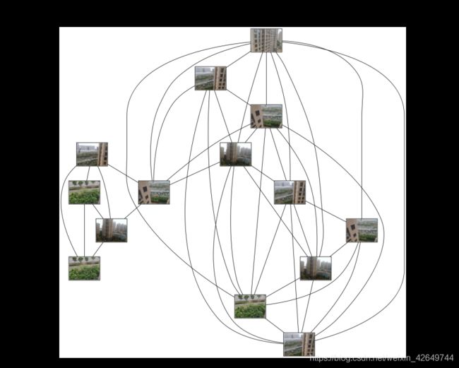
6.3 结果分析
其中连线表示两张图片的匹配度比较高,矩阵保存的是数据集中图片两两进行匹配的匹配数。从图中可以清楚的看到匹配的结果, 此次实验我们设置一个阈值,如果匹配的数目高于一个阈值,我们使用连接线来连接相应的图像。我的数据集数据因为一张像素太大删了一张有十四张图片,可视化连接匹配连接了十三张,说明还有一张是是没有达到阈值的。总体来说,在本组数据集下,匹配准确率较高。
6.4错误分析
(1)安装graphviz时,环境变量添加错误,改正后不报错。
(2)运行过程中因为图片过大 导致运行速度太慢,后面删了一张图片,得到实验结果
七,RANSAC算法
7.1概况
RANSAC是改革派:首先假设数据具有某种特性(目的),为了达到目的,适当割舍一些现有的数据。RANSAC是“RANdom SAmple Consensus”(随机一致性采样)的缩写,它于1981年由Fischler和Bolles最先提出。该方法是用来找到正确模型来拟合带有噪声数据的迭代方法。给定一个模型,例如点集之间 的单应性矩阵,RANSAC 基本的思想是,数据中包含正确的点和噪声点,合理的模型应该能够在描述正确数据点的同时摒弃噪声点。由于一张图片中像素点数量大,采用最小二乘法运算量大,计算速度慢,因此采用RANSAC方法。RANSAC参考:https://www.cnblogs.com/xingshansi/p/6763668.html
ransac
def ransac(data, model, n, k, t, d, debug=False, return_all=False)
参考:http://scipy.github.io/old-wiki/pages/Cookbook/RANSAC
伪代码:http://en.wikipedia.org/w/index.php?title=RANSAC&oldid=116358182
7.2算法步骤
输入:
data - 样本点
model - 假设模型:事先自己确定
n - 生成模型所需的最少样本点
k - 最大迭代次数
t - 阈值:作为判断点满足模型的条件
d - 拟合较好时,需要的样本点最少的个数,当做阈值看待
输出:
bestfit - 最优拟合解(返回nil,如果未找到)
RANSAC 求解单应性矩阵
•RANSAC loop:
随机选择四对匹配特征
根据DLT计算单应矩阵 H (唯一解)
对所有匹配点,计算映射误差ε= ||pi’, H pi||
根据误差阈值,确定inliers(例如3-5像素)
针对最大inliers集合,重新计算单应矩阵 H
7.3代码
import cv2
import numpy as np
import random

def compute_fundamental(x1, x2):

    n = x1.shape[1]

    if x2.shape[1] != n:

        raise ValueError("Number of points don't match.")

    # build matrix for equations

    A = np.zeros((n, 9))

    for i in range(n):

        A[i] = [x1[0, i] * x2[0, i], x1[0, i] * x2[1, i], x1[0, i] * x2[2, i],

                x1[1, i] * x2[0, i], x1[1, i] * x2[1, i], x1[1, i] * x2[2, i],

                x1[2, i] * x2[0, i], x1[2, i] * x2[1, i], x1[2, i] * x2[2, i]]

    # compute linear least square solution

    U, S, V = np.linalg.svd(A)

    F = V[-1].reshape(3, 3)

    # constrain F

    # make rank 2 by zeroing out last singular value

    U, S, V = np.linalg.svd(F)

    S[2] = 0

    F = np.dot(U, np.dot(np.diag(S), V))

    return F / F[2, 2]


def compute_fundamental_normalized(x1, x2):


    n = x1.shape[1]

    if x2.shape[1] != n:

        raise ValueError("Number of points don't match.")

    # normalize image coordinates

    x1 = x1 / x1[2]

    mean_1 = np.mean(x1[:2], axis=1)

    S1 = np.sqrt(2) / np.std(x1[:2])

    T1 = np.array([[S1, 0, -S1 * mean_1[0]], [0, S1, -S1 * mean_1[1]], [0, 0, 1]])

    x1 = np.dot(T1, x1)

    x2 = x2 / x2[2]

    mean_2 = np.mean(x2[:2], axis=1)

    S2 = np.sqrt(2) / np.std(x2[:2])

    T2 = np.array([[S2, 0, -S2 * mean_2[0]], [0, S2, -S2 * mean_2[1]], [0, 0, 1]])

    x2 = np.dot(T2, x2)

    # compute F with the normalized coordinates

    F = compute_fundamental(x1, x2)

    # print (F)

    # reverse normalization

    F = np.dot(T1.T, np.dot(F, T2))

    return F / F[2, 2]

def randSeed(good, num = 8):


    four_point = random.sample(good, num)

    return four_point

def PointCoordinates(eight_points, keypoints1, keypoints2):


    x1 = []

    x2 = []

    tuple_dim = (1.,)

    for i in eight_points:

        tuple_x1 = keypoints1[i[0].queryIdx].pt + tuple_dim

        tuple_x2 = keypoints2[i[0].trainIdx].pt + tuple_dim

        x1.append(tuple_x1)

        x2.append(tuple_x2)

    return np.array(x1, dtype=float), np.array(x2, dtype=float)

def ransac(good, keypoints1, keypoints2, confidence,iter_num):

    Max_num = 0

    good_F = np.zeros([3,3])

    inlier_points = []

    for i in range(iter_num):

        eight_points = randSeed(good)

        x1,x2 = PointCoordinates(eight_points, keypoints1, keypoints2)

        F = compute_fundamental_normalized(x1.T, x2.T)

        num, ransac_good = inlier(F, good, keypoints1, keypoints2, confidence)

        if num > Max_num:

            Max_num = num

            good_F = F

            inlier_points = ransac_good

    print(Max_num, good_F)

    return Max_num, good_F, inlier_points


def computeReprojError(x1, x2, F):


    ww = 1.0/(F[2,0]*x1[0]+F[2,1]*x1[1]+F[2,2])

    dx = (F[0,0]*x1[0]+F[0,1]*x1[1]+F[0,2])*ww - x2[0]

    dy = (F[1,0]*x1[0]+F[1,1]*x1[1]+F[1,2])*ww - x2[1]

    return dx*dx + dy*dy


def inlier(F,good, keypoints1,keypoints2,confidence):

    num = 0

    ransac_good = []

    x1, x2 = PointCoordinates(good, keypoints1, keypoints2)

    for i in range(len(x2)):

        line = F.dot(x1[i].T)


        line_v = np.array([-line[1], line[0]])

        err = h = np.linalg.norm(np.cross(x2[i,:2], line_v)/np.linalg.norm(line_v))

        # err = computeReprojError(x1[i], x2[i], F)

        if abs(err) < confidence:

            ransac_good.append(good[i])

            num += 1

    return num, ransac_good


if __name__ =='__main__':

    im1 = 'C:/Users/59287\Desktop/sift-data/8.jpg'

    im2 = 'C:/Users/59287\Desktop/sift-data/9.jpg'


    print(cv2.__version__)

    psd_img_1 = cv2.imread(im1, cv2.IMREAD_COLOR)

    psd_img_2 = cv2.imread(im2, cv2.IMREAD_COLOR)


    sift = cv2.xfeatures2d.SIFT_create()

    # find the keypoints and descriptors with SIFT

    kp1, des1 = sift.detectAndCompute(psd_img_1, None)

    kp2, des2 = sift.detectAndCompute(psd_img_2, None)


    match = cv2.BFMatcher()

    matches = match.knnMatch(des1, des2, k=2)


    good = []

    for m, n in matches:

        if m.distance < 0.75 * n.distance:

            good.append([m])

    print(good[0][0])


    print("number of feature points:",len(kp1), len(kp2))

    print(type(kp1[good[0][0].queryIdx].pt))

    print("good match num:{} good match points:".format(len(good)))

    for i in good:

        print(i[0].queryIdx, i[0].trainIdx)


    Max_num, good_F, inlier_points = ransac(good, kp1, kp2, confidence=30, iter_num=500)


    img3 = cv2.drawMatchesKnn(psd_img_1,kp1,psd_img_2,kp2,good,None,flags=2)

    img4 = cv2.drawMatchesKnn(psd_img_1,kp1,psd_img_2,kp2,inlier_points,None,flags=2)

    cv2.namedWindow('image1', cv2.WINDOW_NORMAL)

    cv2.namedWindow('image2', cv2.WINDOW_NORMAL)

    cv2.imshow("image1",img3)

    cv2.imshow("image2",img4)

    cv2.waitKey(0)

    cv2.destroyAllWindows()
7.4实验结果

7.5实验小结:
之前实验因为图片像素太大,改小了像素,所以图片比较模糊。此次实验我用了两图片,一组景深丰富,一组景深单一。由实验结果可以知道景深丰富会产生比较多的匹配点,未用过RANSAC算法错误匹配点比较多,用过后错误匹配点明显比较少。但是在景深比较单一的情况下,错误匹配点在未用RANSAC算法就比较少。除此之外RANSAC 算法的优点是能鲁棒的估计模型参数。例如,他能从包含大量局外点的数据集中估计出高精度的参数。缺点是它计算参数的迭代次数没有上限,如果设置迭代次数的上限,得到的结果可能不是最优的结果,甚至可能得到错误的结果。RANSAC只有一定的概率得到的可信的模型,概率与迭代次数成正比。另一个缺点是它要求设置跟问题相关的阈值,RANSAC职能从特定的数据集中估计出一个模型,如果存在两个(或多个)模型,RANSAC不能找到别的模型
八实验小结
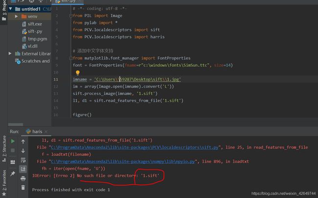
8.1 实验过程中的错误以及解决方法
(1)安装Vlfeat没安装好一直报错,后面发现是Anaconda文件夹下的PCV (我的PCV位置C:ProgramData\Anaconda\Anaconda2\Lib\site-packages\PCV)文件夹里面的localdescriptors文件夹中的sift.py文件,修改的cmmd内的路径时,路径 cmmd =str(r"D:\PythonWork\SIFT\sift.exe “+ imagename+”–output=” + resultname+" "+params) sift.exe后面没加空格
(2)因为电脑没有显卡,运行速度很慢,后面发现是图片像素太大,修改后解决
8.2 SIFT的缺点
SIFT在图像的不变特征提取方面拥有无与伦比的优势,但并不完美,仍然存在:
实时性不高。 有时特征点较少。对边缘光滑的目标无法准确提取特征点。
8.3 对比Harris算子
从匹配的准确率看来,harris算法的结果存在一些不正确的匹配,而sift算法几乎没有匹配错误。显而易见地,sift算法具有较高的准确度及稳健性(对图片亮度不敏感);
从时间上来说,sift算法的效率远高与harris算法,所以sift算法具有更高的计算效率;
总的来说,两个算法由于选择特征点的方法不同,而显示出了差异。sift算法综合了许多前人已经整理出的算法的优点,最后才得到了现在的算法(更优)。