CS224n课程Assignment2参考答案
A s s i g n m e n t # 2 − s o l u t i o n B y J o n a r i g u e z Assignment\#2 -solution\quad By\ Jonariguez Assignment#2−solutionBy Jonariguez
所有的代码题目对应的代码已上传至github/CS224n/Jonariguez
解:
(提示使用keepdims参数会方便一些哦。 )
def softmax(x):
    """
    Compute the softmax function in tensorflow.

    You might find the tensorflow functions tf.exp, tf.reduce_max,
    tf.reduce_sum, tf.expand_dims useful. (Many solutions are possible, so you may
    not need to use all of these functions). Recall also that many common
    tensorflow operations are sugared (e.g. x * y does a tensor multiplication
    if x and y are both tensors). Make sure to implement the numerical stability
    fixes as in the previous homework!

    Args:
        x:   tf.Tensor with shape (n_samples, n_features). Note feature vectors are
                  represented by row-vectors. (For simplicity, no need to handle 1-d
                  input as in the previous homework)
    Returns:
        out: tf.Tensor with shape (n_sample, n_features). You need to construct this
                  tensor in this problem.
    """

    ### YOUR CODE HERE
    """
    跟作业1一样,要先减去每行的最大值,然后再做softmax
    用keepdims=True可以保持之前的形状,而不会变成行向量
    """
    x_max = tf.reduce_max(x,axis=1,keepdims=True)
    x = tf.exp(x-x_max)
    x_sum = tf.reduce_sum(x,axis=1,keepdims=True)
    out = x/x_sum
    #out = x/tf.reshape(tf.reduce_sum(x,axis=1),(x.shape[0],1))
    ### END YOUR CODE

    return out

解:
(积累知识:
- tf.multiply()为元素级的乘法,要求形状相同。
- tf.matmul()为矩阵乘法。
两者都要求两个矩阵的元素类型必须相同。
)
def cross_entropy_loss(y, yhat):
    """
    Compute the cross entropy loss in tensorflow.
    The loss should be summed over the current minibatch.

    y is a one-hot tensor of shape (n_samples, n_classes) and yhat is a tensor
    of shape (n_samples, n_classes). y should be of dtype tf.int32, and yhat should
    be of dtype tf.float32.

    The functions tf.to_float, tf.reduce_sum, and tf.log might prove useful. (Many
    solutions are possible, so you may not need to use all of these functions).

    Note: You are NOT allowed to use the tensorflow built-in cross-entropy
                functions.

    Args:
        y:    tf.Tensor with shape (n_samples, n_classes). One-hot encoded.
        yhat: tf.Tensorwith shape (n_sample, n_classes). Each row encodes a
                    probability distribution and should sum to 1.
    Returns:
        out:  tf.Tensor with shape (1,) (Scalar output). You need to construct this
                    tensor in the problem.
    """

    ### YOUR CODE HERE
    """
    y和y_hat的第一维都是n_samples,这是一个batch的大小,也即batch_size,那么对于
    每一个sample都要计算一个交叉熵(标量,实数),然后再把这n_samples个交叉熵求和,最终也是个标量(实数)
    """
    single_CE = tf.multiply(tf.log(yhat),tf.to_float(y))
    out = tf.negative(tf.reduce_sum(single_CE))
    ### END YOUR CODE

    return out
解:
占位符(placeholder)和feed_dict可以在运行时动态地向计算图“喂”数据。(TensorFlow采用的是静态图)
def add_placeholders(self):
    """Generates placeholder variables to represent the input tensors.

    These placeholders are used as inputs by the rest of the model building
    and will be fed data during training.

    Adds following nodes to the computational graph

    input_placeholder: Input placeholder tensor of shape
                                          (batch_size, n_features), type tf.float32
    labels_placeholder: Labels placeholder tensor of shape
                                          (batch_size, n_classes), type tf.int32

    Add these placeholders to self as the instance variables
        self.input_placeholder
        self.labels_placeholder
    """
    ### YOUR CODE HERE
    self.input_placeholder = tf.placeholder(tf.float32,shape=[self.config.batch_size,self.config.n_features],name='input_placeholder')
    self.labels_placeholder = tf.placeholder(tf.int32,shape=[self.config.batch_size,self.config.n_classes],name='labels_placeholder')
    ### END YOUR CODE
def create_feed_dict(self, inputs_batch, labels_batch=None):
    """Creates the feed_dict for training the given step.

    A feed_dict takes the form of:
    feed_dict = {
            : ,
            ....
    }

    If label_batch is None, then no labels are added to feed_dict.

    Hint: The keys for the feed_dict should be the placeholder
            tensors created in add_placeholders.

    Args:
        inputs_batch: A batch of input data.
        labels_batch: A batch of label data.
    Returns:
        feed_dict: The feed dictionary mapping from placeholders to values.
    """
    ### YOUR CODE HERE
    """
    feed_dict其实就是python里面字典类型
    注意:feed_dict的键是我们之前定义过的tf.placeholder对象,而不是tf.placeholder的str类型的名字
    """
    feed_dict = {
        self.input_placeholder:inputs_batch,
        self.labels_placeholder:labels_batch
    }
    ### END YOUR CODE
    return feed_dict

def add_prediction_op(self):
     """Adds the core transformation for this model which transforms a batch of input
     data into a batch of predictions. In this case, the transformation is a linear layer plus a
     softmax transformation:

     y = softmax(Wx + b)

     Hint: Make sure to create tf.Variables as needed.
     Hint: For this simple use-case, it's sufficient to initialize both weights W
                 and biases b with zeros.

     Args:
         input_data: A tensor of shape (batch_size, n_features).
     Returns:
         pred: A tensor of shape (batch_size, n_classes)
     """
     ### YOUR CODE HERE
     """
     x是输入,即占位符input_placeholder
     而W和b是要定义的变量,也是要训练的变量
     pred = softmax(xW+b)
     """
     with tf.variable_scope('softmax_classifier'):
         W = tf.Variable(tf.zeros([self.config.n_features,self.config.n_classes],dtype=tf.float32))
         b = tf.Variable(tf.zeros([self.config.n_classes],dtype=tf.float32))
         # print(W.name)
         # print(b.name)
         Z = tf.matmul(self.input_placeholder,W)+b
         pred = softmax(Z)
     ### END YOUR CODE
     return pred
def add_loss_op(self, pred):
        """Adds cross_entropy_loss ops to the computational graph.

        Hint: Use the cross_entropy_loss function we defined. This should be a very
                    short function.
        Args:
            pred: A tensor of shape (batch_size, n_classes)
        Returns:
            loss: A 0-d tensor (scalar)
        """
        ### YOUR CODE HERE
        """
        因为我们已经在q1_softmax.py中定义并实现了cross_entropy_loss()函数,所以这里可以直接调用
        self.labels_placeholder 是"喂"进来的真实标记
        pred    是我们预测的
        """
        loss = cross_entropy_loss(self.labels_placeholder,pred)
        ### END YOUR CODE
        return loss
def add_training_op(self, loss):
    """Sets up the training Ops.

    Creates an optimizer and applies the gradients to all trainable variables.
    The Op returned by this function is what must be passed to the
    `sess.run()` call to cause the model to train. See

    https://www.tensorflow.org/versions/r0.7/api_docs/python/train.html#Optimizer

    for more information.

    Hint: Use tf.train.GradientDescentOptimizer to get an optimizer object.
                Calling optimizer.minimize() will return a train_op object.

    Args:
        loss: Loss tensor, from cross_entropy_loss.
    Returns:
        train_op: The Op for training.
    """
    ### YOUR CODE HERE
    #直接返回优化器即可
    train_op = tf.train.GradientDescentOptimizer(self.config.lr).minimize(loss)
    ### END YOUR CODE
    return train_op
解:
TensorFlow的自动梯度,是指我们使用时只需要定义图的节点就好了,不用自己实现求解梯度,反向传播和求导由TensorFlow自动完成。
解:
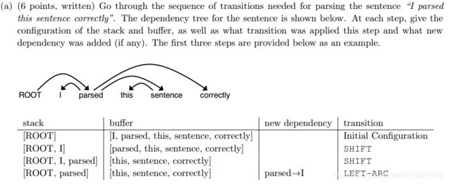
| stack | buffer | new dependency | transition |
|---|---|---|---|
| [ROOT,parsed,this] | [sentence,correctly] | SHIFT | |
| [ROOT,parsed,this,sentence] | [correctly] | SHIFT | |
| [ROOT,parsed,sentence] | [correctly] | sentence -> this | LEFT-ARC |
| [ROOT,parsed] | [correctly] | parsed -> sentence | RIGHT-ARC |
| [ROOT,parsed,correctly] | [] | SHIFT | |
| [ROOT,parsed] | [] | parsed -> correctly | RIGHT-ARC |
| [ROOT] | [] | ROOT -> parsed | RIGHT-ARC |
![]()
解:
共2n步
- 每个词都要进入stack中,故要有n步SHIFT操作。
- 最终stack中只剩ROOT,即每一次ARC会从stack中删掉一个词,故共有n步LEFT-ARC和RIGHT-ARC操作。

def __init__(self, sentence):
    """Initializes this partial parse.

    Your code should initialize the following fields:
        self.stack: The current stack represented as a list with the top of the stack as the
                    last element of the list.
        self.buffer: The current buffer represented as a list with the first item on the
                     buffer as the first item of the list
        self.dependencies: The list of dependencies produced so far. Represented as a list of
                tuples where each tuple is of the form (head, dependent).
                Order for this list doesn't matter.

    The root token should be represented with the string "ROOT"

    Args:
        sentence: The sentence to be parsed as a list of words.
                  Your code should not modify the sentence.
    """
    # The sentence being parsed is kept for bookkeeping purposes. Do not use it in your code.
    self.sentence = sentence

    ### YOUR CODE HERE
    self.stack = ['ROOT']
    #注意不要用self.buffer=sentence,因为这样的话self.buffer是sentence的一个
    #引用,改变self.buffer的话就是直接改变sentence,这和题目要求不符(Do not use it in your code)
    self.buffer = [word for word in self.sentence]
    self.dependencies = []
    ### END YOUR CODE

def parse_step(self, transition):
        """Performs a single parse step by applying the given transition to this partial parse

        Args:
            transition: A string that equals "S", "LA", or "RA" representing the shift, left-arc,
                        and right-arc transitions.
        """
        ### YOUR CODE HERE
        """
        重申一下操作:
        S   从buffer的最左边取出一个word,放入stack最右边
        LA  将stack最右边的word作为head,第二个word作为dependent
        RA  将stack最右边的word作为dependent,第二个word作为head
        LA和RA操作都在self.dependencies中添加(head,dependent)元组
        利用list的pop()函数具有返回值的特性可以简化代码
        """
        if transition=='S':
            self.stack.append(self.buffer.pop(0))
        elif transition=='LA':
            dependent = (self.stack[-1],self.stack.pop(-2))
            self.dependencies.append(dependent)
        else :
            dependent = (self.stack[-2],self.stack.pop(-1))
            self.dependencies.append(dependent)
        ### END YOUR CODE
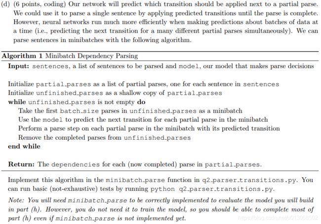

def minibatch_parse(sentences, model, batch_size):
    """Parses a list of sentences in minibatches using a model.

    Args:
        sentences: A list of sentences to be parsed (each sentence is a list of words)
        model: The model that makes parsing decisions. It is assumed to have a function
               model.predict(partial_parses) that takes in a list of PartialParses as input and
               returns a list of transitions predicted for each parse. That is, after calling
                   transitions = model.predict(partial_parses)
               transitions[i] will be the next transition to apply to partial_parses[i].
        batch_size: The number of PartialParses to include in each minibatch
    Returns:
        dependencies: A list where each element is the dependencies list for a parsed sentence.
                      Ordering should be the same as in sentences (i.e., dependencies[i] should
                      contain the parse for sentences[i]).
    """

    ### YOUR CODE HERE
    start_idx,end_idx=0,0
    PartialParses = [PartialParse(sentence) for sentence in sentences]
    dependencies = []
    while end_idx<len(sentences):
        end_idx = min(start_idx+batch_size,len(sentences))
        #拿到batch_size的PartialParse
        #对于每一个句子创建一个PartialParse解析器
        batch_PartialParses = PartialParses[start_idx:end_idx]
        #然后用模型预测,得出每一个句子的transition(transitions[i])
        #注意:model.predict(x)只会对x里面的每一个解析器推进一步。
        while len(batch_PartialParses)>0:
            transitions = model.predict(batch_PartialParses)
            for i in range(len(transitions)):
                batch_PartialParses[i].parse_step(transitions[i])
            #然后把那么句子已经解析完成的丢掉,保留还没有完成的。
            #那么那些是已经完成了的呢?那就是buffer==0 && stack==1
            batch_PartialParses = [parse for parse in batch_PartialParses if len(parse.buffer)>0 or len(parse.stack)>1]

        dependencies.extend([parse.dependencies for parse in PartialParses[start_idx:end_idx]])
        #注意更新start_idx
        start_idx+=batch_size
    ### END YOUR CODE

    return dependencies

def xavier_weight_init():
    """Returns function that creates random tensor.

    The specified function will take in a shape (tuple or 1-d array) and
    returns a random tensor of the specified shape drawn from the
    Xavier initialization distribution.

    Hint: You might find tf.random_uniform useful.
    """
    def _xavier_initializer(shape, **kwargs):
        """Defines an initializer for the Xavier distribution.
        Specifically, the output should be sampled uniformly from [-epsilon, epsilon] where
            epsilon = sqrt(6) /
        e.g., if shape = (2, 3), epsilon = sqrt(6 / (2 + 3))

        This function will be used as a variable initializer.

        Args:
            shape: Tuple or 1-d array that species the dimensions of the requested tensor.
        Returns:
            out: tf.Tensor of specified shape sampled from the Xavier distribution.
        """
        ### YOUR CODE HERE
        epsilon = tf.sqrt(6.0/tf.to_float(tf.reduce_sum(shape)))
        out = tf.Variable(tf.random_uniform(shape,minval=-epsilon,maxval=epsilon))
        ### END YOUR CODE
        return out
    # Returns defined initializer function.
    return _xavier_initializer

解:
E p d r o p [ h d r o p ] = E p d r o p [ γ d ∘ h ] = p d r o p ⋅ 0 ⃗ + ( 1 − p d r o p ) ⋅ γ ⋅ h = h \mathbb{E}_{p_{drop}}[\mathbf{h}_{drop}]=\mathbb{E}_{p_{drop}}[\gamma \mathbf{d}\circ \mathbf{h}]=p_{drop}\cdot \vec{0}+(1-p_{drop})\cdot\gamma\cdot\mathbf{h}=\mathbf{h} Epdrop[hdrop]=Epdrop[γd∘h]=pdrop⋅0+(1−pdrop)⋅γ⋅h=h
即推导出:
γ = 1 1 − p d r o p \gamma=\frac{1}{1-p_{drop}} γ=1−pdrop1
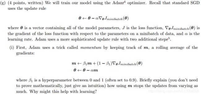
解:
因为其实 m \mathbf{m} m是之前全部梯度(更新量)的加权平均,更能体现梯度的整体变化。因为这样减小了更新量的方差,避免了梯度振荡。
β 1 \mathbf{\beta_1} β1一般要接近1。
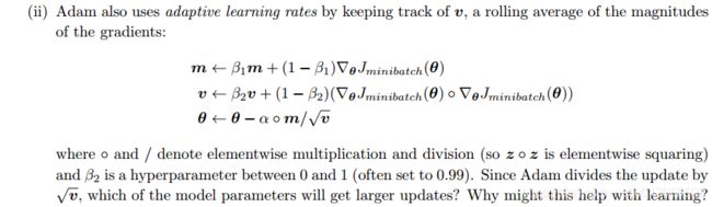
解:
- 更新量 m \mathbf{m} m: 对梯度(更新量)进行滑动平均
- 学习率 v \mathbf{v} v: 对梯度的平方进行滑动平均
梯度平均最小的参数的更新量最大,也就是说,在损失函数相对于它们的梯度很小的时候也能快速收敛。即在平缓的地方也能快递移动到最优解。
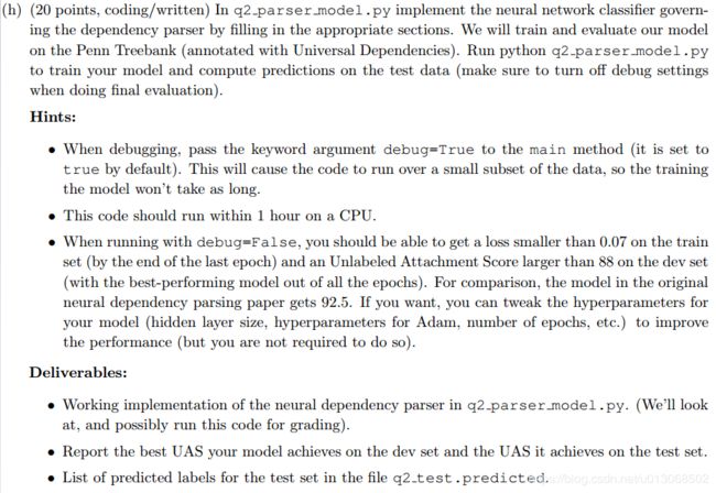
解:
我的结果为
Epoch 10 out of 10
924/924 [============================>.] - ETA: 0s - train loss: 0.0654
Evaluating on dev set - dev UAS: 88.37
New best dev UAS! Saving model in ./data/weights/parser.weights

===========================================================================
TESTING
===========================================================================
Restoring the best model weights found on the dev set
Final evaluation on test set
- test UAS: 88.84
运行时间:15分钟。

题目解读
先明确题目中各个量的维度:
由题目可知, x ( t ) x^{(t)} x(t)是one-hot行向量,且隐藏层也是行向量的形式。
则可得:
x ( t ) ∈ R 1 × ∣ V ∣ x^{(t)}\in \mathbb{R}^{1\times |V|} x(t)∈R1×∣V∣
h ( t ) ∈ R 1 × D h h^{(t)}\in \mathbb{R}^{1\times D_h} h(t)∈R1×Dh
y ^ ( t ) \hat{y}^{(t)} y^(t)是输出,即每个单词的概率分布(softmax之后),那么:
y ^ ( t ) ∈ R 1 × ∣ V ∣ \hat{y}^{(t)}\in \mathbb{R}^{1\times |V|} y^(t)∈R1×∣V∣
然后我们就可以得到:
L ∈ R ∣ V ∣ × d L\in \mathbb{R}^{|V|\times d} L∈R∣V∣×d
e ( t ) ∈ R 1 × d e^{(t)}\in \mathbb{R}^{1\times d} e(t)∈R1×d
I ∈ R d × D h I\in \mathbb{R}^{d\times D_h} I∈Rd×Dh
H ∈ R D h × D h H\in \mathbb{R}^{D_h\times D_h} H∈RDh×Dh
b 1 ∈ R 1 × D h b_1\in \mathbb{R}^{1\times D_h} b1∈R1×Dh
U ∈ R D h × ∣ V ∣ U\in \mathbb{R}^{D_h\times |V|} U∈RDh×∣V∣
b 2 ∈ R 1 × ∣ V ∣ b_2\in \mathbb{R}^{1\times |V|} b2∈R1×∣V∣
其中 d d d是词向量的长度,也就是代码中的 e m b e d _ s i z e embed\_size embed_size。
在清楚了上面各矩阵的维度之后的求导才会更清晰。
因为句子的长度不一,然后损失函数是针对一个单词所计算的,然后求和之后是对整个句子的损失,故要对损失函数求平均以得到每个单词的平均损失才行。
解:
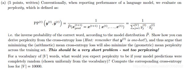
由于标签 y ( t ) y^{(t)} y(t)是one-hot向量,假设 y ( t ) y^{(t)} y(t)的真实标记为 k k k
则:
J ( t ) ( θ ) = C E ( y ( t ) , y ^ ( t ) ) = − l o g y ^ k ( t ) = l o g 1 y ^ k ( t ) J^{(t)}(\theta)=CE(y^{(t)},\hat{y}^{(t)})=-log\ \hat{y}_k^{(t)}=log\ \frac{1}{\hat{y}_k^{(t)}} J(t)(θ)=CE(y(t),y^(t))=−log y^k(t)=log y^k(t)1
P P ( t ) ( y ( t ) , y ^ ( t ) ) = 1 y ^ k ( t ) PP^{(t)}(y^{(t)},\hat{y}^{(t)})=\frac{1}{\hat{y}_k^{(t)}} PP(t)(y(t),y^(t))=y^k(t)1
很容易得出:
C E ( y ( t ) , y ^ ( t ) ) = l o g P P ( t ) ( y ( t ) , y ^ ( t ) ) CE(y^{(t)},\hat{y}^{(t)})=log\ PP^{(t)}(y^{(t)},\hat{y}^{(t)}) CE(y(t),y^(t))=log PP(t)(y(t),y^(t))
很常见的结论,一定要知道的。
当 ∣ V ∣ = 10000 |V|=10000 ∣V∣=10000时,随机选择能选对的概率为 1 ∣ V ∣ = 1 10000 \frac{1}{|V|}=\frac{1}{10000} ∣V∣1=100001, p e r p l e x i t y perplexity perplexity(困惑度)为 1 1 ∣ V ∣ = 10000 \frac{1}{\frac{1}{|V|}}=10000 ∣V∣11=10000。 C E = l o g 10000 ≈ 9.21 CE=log10000\thickapprox 9.21 CE=log10000≈9.21。

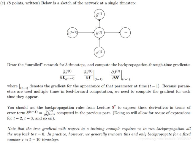
解:
根据题目可知: L x ( t ) = e ( t ) L_{x^{(t)}}=e^{(t)} Lx(t)=e(t)。
现在设:
v ( t ) = h ( t − 1 ) H + e ( t ) I + b 1 v^{(t)}=h^{(t-1)}H+e^{(t)}I+b_1 v(t)=h(t−1)H+e(t)I+b1
θ ( t ) = h ( t ) U + b 2 \theta^{(t)}=h^{(t)}U+b_2 θ(t)=h(t)U+b2
则前向传播为:
e ( t ) = x ( t ) L e^{(t)}=x^{(t)}L e(t)=x(t)L
v ( t ) = h ( t − 1 ) H + e ( t ) I + b 1 v^{(t)}=h^{(t-1)}H+e^{(t)}I+b_1 v(t)=h(t−1)H+e(t)I+b1
h ( t ) = s i g m o i d ( v ( t ) ) h^{(t)}=sigmoid(v^{(t)}) h(t)=sigmoid(v(t))
θ ( t ) = h ( t ) U + b 2 \theta^{(t)}=h^{(t)}U+b_2 θ(t)=h(t)U+b2
y ^ ( t ) = s o f t m a x ( θ ( t ) ) \hat{y}^{(t)}=softmax(\theta^{(t)}) y^(t)=softmax(θ(t))
J ( t ) = C E ( y ( t ) , y ^ ( t ) ) J^{(t)}=CE(y^{(t)},\hat{y}^{(t)}) J(t)=CE(y(t),y^(t))
反向传播:
中间值:
δ 1 ( t ) = ∂ J ( t ) ∂ θ ( t ) = y ^ ( t ) − y ( t ) \delta_1^{(t)}=\frac{\partial J^{(t)}}{\partial \theta^{(t)}}=\hat{y}^{(t)}-y^{(t)} δ1(t)=∂θ(t)∂J(t)=y^(t)−y(t)
δ 2 ( t ) = ∂ J ( t ) ∂ v ( t ) = ∂ J ( t ) ∂ θ ( t ) ⋅ ∂ θ ( t ) ∂ h ( t ) ⋅ ∂ h ( t ) ∂ v ( t ) = ( y ^ ( t ) − y ( t ) ) ⋅ U T ∘ h ( t ) ∘ ( 1 − h ( t ) ) \delta_2^{(t)}=\frac{\partial J^{(t)}}{\partial v^{(t)}}=\frac{\partial J^{(t)}}{\partial \theta^{(t)}}\cdot\frac{\partial \theta^{(t)}}{\partial h^{(t)}}\cdot\frac{\partial h^{(t)}}{\partial v^{(t)}}=(\hat{y}^{(t)}-y^{(t)})\cdot U^{T}\circ h^{(t)}\circ (1-h^{(t)}) δ2(t)=∂v(t)∂J(t)=∂θ(t)∂J(t)⋅∂h(t)∂θ(t)⋅∂v(t)∂h(t)=(y^(t)−y(t))⋅UT∘h(t)∘(1−h(t))
则有:
∂ J ( t ) ∂ b 2 = ∂ J ( t ) ∂ θ ( t ) ⋅ ∂ θ ( t ) ∂ b 2 = δ 1 ( t ) \frac{\partial J^{(t)}}{\partial b_2}=\frac{\partial J^{(t)}}{\partial \theta^{(t)}}\cdot\frac{\partial \theta^{(t)}}{\partial b_2}=\delta_1^{(t)} ∂b2∂J(t)=∂θ(t)∂J(t)⋅∂b2∂θ(t)=δ1(t)
∂ J ( t ) ∂ H ∣ t = ∂ J ( t ) ∂ v ( t ) ∂ v ( t ) ∂ H ∣ t = ( h ( t − 1 ) ) T ⋅ δ 2 ( t ) \frac{\partial J^{(t)}}{\partial H}\rvert_t = \frac{\partial J^{(t)}}{\partial v^{(t)}}\frac{\partial v^{(t)}}{\partial H}\rvert_t=(h^{(t-1)})^T\cdot\delta_2^{(t)} ∂H∂J(t)∣t=∂v(t)∂J(t)∂H∂v(t)∣t=(h(t−1))T⋅δ2(t)
∂ J ( t ) ∂ I ∣ t = ∂ J ( t ) ∂ v ( t ) ∂ v ( t ) ∂ I ∣ t = ( e ( t ) ) T ⋅ δ 2 ( t ) \frac{\partial J^{(t)}}{\partial I}\rvert_t = \frac{\partial J^{(t)}}{\partial v^{(t)}}\frac{\partial v^{(t)}}{\partial I}\rvert_t=(e^{(t)})^T\cdot\delta_2^{(t)} ∂I∂J(t)∣t=∂v(t)∂J(t)∂I∂v(t)∣t=(e(t))T⋅δ2(t)
∂ J ( t ) ∂ L x ( t ) = ∂ J ( t ) ∂ e ( t ) = ∂ J ( t ) ∂ v ( t ) ⋅ ∂ v ( t ) ∂ e ( t ) = δ 2 ( t ) ⋅ I T \frac{\partial J^{(t)}}{\partial L_{x^{(t)}}} =\frac{\partial J^{(t)}}{\partial e^{(t)}}= \frac{\partial J^{(t)}}{\partial v^{(t)}}\cdot \frac{\partial v^{(t)}}{\partial e^{(t)}}=\delta_2^{(t)}\cdot I^T ∂Lx(t)∂J(t)=∂e(t)∂J(t)=∂v(t)∂J(t)⋅∂e(t)∂v(t)=δ2(t)⋅IT
∂ J ( t ) ∂ h ( t − 1 ) = ∂ J ( t ) ∂ v ( t ) ⋅ ∂ v ( t ) ∂ h ( t − 1 ) = δ 2 ( t ) ⋅ H T \frac{\partial J^{(t)}}{\partial h^{(t-1)}}= \frac{\partial J^{(t)}}{\partial v^{(t)}}\cdot \frac{\partial v^{(t)}}{\partial h^{(t-1)}}=\delta_2^{(t)}\cdot H^T ∂h(t−1)∂J(t)=∂v(t)∂J(t)⋅∂h(t−1)∂v(t)=δ2(t)⋅HT
如果你对上面的反向传播中的求导有疑惑,那么请看下面的简单讲解
考虑如下求导:
∂ J ∂ x = ∂ J ∂ u 1 ∂ u 1 ∂ u 2 ⋅ ⋅ ⋅ ⋅ ∂ u m ∂ v ∂ v ∂ x \frac{\partial J}{\partial x}=\frac{\partial J}{\partial u_1}\frac{\partial u_1}{\partial u_2}\cdot\cdot\cdot\cdot\frac{\partial u_{m}}{\partial v}\frac{\partial v}{\partial x} ∂x∂J=∂u1∂J∂u2∂u1⋅⋅⋅⋅∂v∂um∂x∂v
假设除了 ∂ v ∂ x \frac{\partial v}{\partial x} ∂x∂v,前面的已经求出了
∂ J ∂ u 1 ∂ u 1 ∂ u 2 ⋅ ⋅ ⋅ ⋅ ∂ u m ∂ v = δ \frac{\partial J}{\partial u_1}\frac{\partial u_1}{\partial u_2}\cdot\cdot\cdot\cdot\frac{\partial u_{m}}{\partial v}=\delta ∂u1∂J∂u2∂u1⋅⋅⋅⋅∂v∂um=δ
现在就差 ∂ v ∂ x \frac{\partial v}{\partial x} ∂x∂v了。需要讨论两种情况:
- 其中, v v v是一个行向量 r r r乘上一个矩阵 M M M,然后对矩阵 M M M求导:
∂ v ∂ x = ∂ ∂ M ( r M ) \frac{\partial v}{\partial x}=\frac{\partial }{\partial M}(rM) ∂x∂v=∂M∂(rM)
结果为 r T r^T rT 左乘 前面一坨的求导结果 δ \delta δ,即:
∂ J ∂ x = r T ⋅ δ \frac{\partial J}{\partial x}=r^T\cdot\delta ∂x∂J=rT⋅δ
而具体到题目中就是:
∂ J ( t ) ∂ v ( t ) = δ 2 ( t ) \frac{\partial J^{(t)}}{\partial v^{(t)}}=\delta_2^{(t)} ∂v(t)∂J(t)=δ2(t)
∂ v ( t ) ∂ H = ∂ ∂ H ( h ( t − 1 ) H + e ( t ) I + b 1 ) = ∂ ∂ H ( h ( t − 1 ) H ) = ( h ( t − 1 ) ) T \frac{\partial v^{(t)}}{\partial H}=\frac{\partial }{\partial H}(h^{(t-1)}H+e^{(t)}I+b_1)=\frac{\partial }{\partial H}(h^{(t-1)}H)=(h^{(t-1)})^T ∂H∂v(t)=∂H∂(h(t−1)H+e(t)I+b1)=∂H∂(h(t−1)H)=(h(t−1))T
所以:
∂ J ( t ) ∂ H ∣ t = ∂ J ( t ) ∂ v ( t ) ∂ v ( t ) ∂ H ∣ t = ( h ( t − 1 ) ) T ⋅ δ 2 ( t ) \frac{\partial J^{(t)}}{\partial H}\rvert_t=\frac{\partial J^{(t)}}{\partial v^{(t)}}\frac{\partial v^{(t)}}{\partial H}\rvert_t=(h^{(t-1)})^T\cdot\delta_2^{(t)} ∂H∂J(t)∣t=∂v(t)∂J(t)∂H∂v(t)∣t=(h(t−1))T⋅δ2(t)
- 其中, v v v是一个行向量 r r r乘上一个矩阵 M M M,然后对行向量 r r r求导:
∂ v ∂ x = ∂ ∂ r ( r M ) \frac{\partial v}{\partial x}=\frac{\partial }{\partial r}(rM) ∂x∂v=∂r∂(rM)
结果为 M T M^T MT 右乘 前面一坨的求导结果 δ \delta δ,即:
∂ J ∂ x = δ ⋅ M T \frac{\partial J}{\partial x}=\delta\cdot M^T ∂x∂J=δ⋅MT
而具体到题目中就是:
∂ J ( t ) ∂ h ( t − 1 ) = ∂ J ( t ) ∂ v ( t ) ⋅ ∂ v ( t ) ∂ h ( t − 1 ) = δ 2 ( t ) ⋅ H T \frac{\partial J^{(t)}}{\partial h^{(t-1)}}= \frac{\partial J^{(t)}}{\partial v^{(t)}}\cdot \frac{\partial v^{(t)}}{\partial h^{(t-1)}}=\delta_2^{(t)}\cdot H^T ∂h(t−1)∂J(t)=∂v(t)∂J(t)⋅∂h(t−1)∂v(t)=δ2(t)⋅HT
解:
RNN的反向传播是按时间的反向传播,对于时间步 t t t的损失函数 J ( t ) J^{(t)} J(t)要沿时间向前传播,故现在为了方便,定义时间步 t t t的损失函数 J ( t ) J^{(t)} J(t)对每一时间步的误差项 δ ( t ) \delta^{(t)} δ(t):
δ ( t ) = ∂ J ( t ) ∂ h ( t ) \delta^{(t)}=\frac{\partial J^{(t)}}{\partial h^{(t)}} δ(t)=∂h(t)∂J(t)
现推导误差项的传播:
δ ( t ) = ∂ J ( t ) ∂ h ( t ) = ( y ^ − y ) ⋅ U T \delta^{(t)}=\frac{\partial J^{(t)}}{\partial h^{(t)}}=(\hat{y}-y)\cdot U^T δ(t)=∂h(t)∂J(t)=(y^−y)⋅UT
h ( t ) = s i g m o i d ( h ( t − 1 ) H + e ( t ) I + b 1 ) h^{(t)}=sigmoid(h^{(t-1)}H+e^{(t)}I+b_1) h(t)=sigmoid(h(t−1)H+e(t)I+b1)
∂ h ( t ) ∂ h ( t − 1 ) = h ( t ) ∘ ( 1 − h ( t ) ) ∘ H T \frac{\partial h^{(t)}}{\partial h^{(t-1)}}=h^{(t)}\circ (1-h^{(t)})\circ H^T ∂h(t−1)∂h(t)=h(t)∘(1−h(t))∘HT
故可得递推式:
δ ( t − 1 ) = ∂ J ( t ) ∂ h ( t − 1 ) = ∂ J ( t ) ∂ h ( t ) ⋅ ∂ h ( t ) ∂ h ( t − 1 ) = δ ( t ) ∘ h ( t ) ∘ ( 1 − h ( t ) ) ⋅ H T \delta^{(t-1)}=\frac{\partial J^{(t)}}{\partial h^{(t-1)}}=\frac{\partial J^{(t)}}{\partial h^{(t)}}\cdot\frac{\partial h^{(t)}}{\partial h^{(t-1)}}=\delta^{(t)}\circ h^{(t)}\circ(1-h^{(t)})\cdot H^T δ(t−1)=∂h(t−1)∂J(t)=∂h(t)∂J(t)⋅∂h(t−1)∂h(t)=δ(t)∘h(t)∘(1−h(t))⋅HT
即可得:
∂ J ( t ) ∂ L x ( t − 1 ) = ∂ J ( t ) ∂ h ( t − 1 ) ⋅ ∂ h ( t − 1 ) ∂ L x ( t − 1 ) = δ ( t − 1 ) ⋅ I T ∘ h ( t − 1 ) ∘ ( 1 − h ( t − 1 ) ) \frac{\partial J^{(t)}}{\partial L_{x^{(t-1)}}}=\frac{\partial J^{(t)}}{\partial h^{(t-1)}}\cdot\frac{\partial h^{(t-1)}}{\partial L_{x^{(t-1)}}}=\delta^{(t-1)}\cdot I^T\circ h^{(t-1)}\circ(1-h^{(t-1)}) ∂Lx(t−1)∂J(t)=∂h(t−1)∂J(t)⋅∂Lx(t−1)∂h(t−1)=δ(t−1)⋅IT∘h(t−1)∘(1−h(t−1))
∂ J ( t ) ∂ I ∣ t − 1 = ∂ J ( t ) ∂ h ( t − 1 ) ⋅ ∂ h ( t − 1 ) ∂ I ∣ t − 1 = ( e ( t − 1 ) ) T ⋅ δ ( t − 1 ) ∘ h ( t − 1 ) ∘ ( 1 − h ( t − 1 ) ) \frac{\partial J^{(t)}}{\partial I}\rvert_{t-1}=\frac{\partial J^{(t)}}{\partial h^{(t-1)}}\cdot\frac{\partial h^{(t-1)}}{\partial I}\rvert_{t-1}=(e^{(t-1)})^T\cdot\delta^{(t-1)}\circ h^{(t-1)}\circ(1-h^{(t-1)}) ∂I∂J(t)∣t−1=∂h(t−1)∂J(t)⋅∂I∂h(t−1)∣t−1=(e(t−1))T⋅δ(t−1)∘h(t−1)∘(1−h(t−1))
∂ J ( t ) ∂ H ∣ t − 1 = ∂ J ( t ) ∂ h ( t − 1 ) ⋅ ∂ h ( t − 1 ) ∂ H ∣ t − 1 = ( h ( t − 2 ) ) T ⋅ δ ( t − 1 ) ∘ h ( t − 1 ) ∘ ( 1 − h ( t − 1 ) ) \frac{\partial J^{(t)}}{\partial H}\rvert_{t-1}=\frac{\partial J^{(t)}}{\partial h^{(t-1)}}\cdot\frac{\partial h^{(t-1)}}{\partial H}\rvert_{t-1}=(h^{(t-2)})^T\cdot\delta^{(t-1)}\circ h^{(t-1)}\circ(1-h^{(t-1)}) ∂H∂J(t)∣t−1=∂h(t−1)∂J(t)⋅∂H∂h(t−1)∣t−1=(h(t−2))T⋅δ(t−1)∘h(t−1)∘(1−h(t−1))
注意,上述过程用到了 s i g m o i d sigmoid sigmoid 函数的导数:
σ ′ ( x ) = σ ( x ) ∘ ( 1 − σ ( x ) ) \sigma'(x)=\sigma(x)\circ(1-\sigma(x)) σ′(x)=σ(x)∘(1−σ(x))
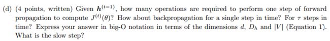
前向传播的复杂度分别为:
e ( t ) = x ( t ) L ⟶ O ( ∣ V ∣ ) e^{(t)}=x^{(t)}L \longrightarrow O(|V|) e(t)=x(t)L⟶O(∣V∣)
v ( t ) = h ( t − 1 ) H + e ( t ) I + b 1 ⟶ O ( D h 2 ) + O ( d D h ) v^{(t)}=h^{(t-1)}H+e^{(t)}I+b_1 \longrightarrow O(D_h^2)+O(dD_h) v(t)=h(t−1)H+e(t)I+b1⟶O(Dh2)+O(dDh)
h ( t ) = s i g m o i d ( v ( t ) ) ⟶ O ( D h ) h^{(t)}=sigmoid(v^{(t)}) \longrightarrow O(D_h) h(t)=sigmoid(v(t))⟶O(Dh)
θ ( t ) = h ( t ) U + b 2 ⟶ O ( ∣ V ∣ D h ) \theta^{(t)}=h^{(t)}U+b_2 \longrightarrow O(|V|D_h) θ(t)=h(t)U+b2⟶O(∣V∣Dh)
y ^ ( t ) = s o f t m a x ( θ ( t ) ) ⟶ O ( ∣ V ∣ ) \hat{y}^{(t)}=softmax(\theta^{(t)}) \longrightarrow O(|V|) y^(t)=softmax(θ(t))⟶O(∣V∣)
J ( t ) = C E ( y ( t ) , y ^ ( t ) ) ⟶ O ( ∣ V ∣ ) J^{(t)}=CE(y^{(t)},\hat{y}^{(t)}) \longrightarrow O(|V|) J(t)=CE(y(t),y^(t))⟶O(∣V∣)
综上,在有两阶的时候则只保留两阶的情况下,前向传播的复杂度为:
O ( D h 2 + d D h + ∣ V ∣ D h ) O(D_h^2+dD_h+|V|D_h) O(Dh2+dDh+∣V∣Dh)
同理,反向传播的复杂度为:
O ( D h 2 + d D h + ∣ V ∣ D h ) O(D_h^2+dD_h+|V|D_h) O(Dh2+dDh+∣V∣Dh)
上述是第一个时间步长的复杂度,而 τ \tau τ个时间步的话就是:
- 一次损失函数对 h ( t ) h^{(t)} h(t)的求导,复杂度为 O ( ∣ V ∣ D h ) O(|V|D_h) O(∣V∣Dh);
- τ \tau τ次反向传播,复杂度为 O ( τ ( D h 2 + d D h ) ) O(\tau(D_h^2+dD_h)) O(τ(Dh2+dDh));
故, τ \tau τ个时间步的反向传播复杂度为:
O ( τ ( D h 2 + d D h ) + ∣ V ∣ D h ) O(\tau(D_h^2+dD_h)+|V|D_h) O(τ(Dh2+dDh)+∣V∣Dh)
而如果是对前 τ \tau τ个词,每次都进行 τ \tau τ步的反向传播,那么复杂度大概为:
O ( τ 2 ( D h 2 + d D h ) + τ ∣ V ∣ D h ) O(\tau^2(D_h^2+dD_h)+\tau|V|D_h) O(τ2(Dh2+dDh)+τ∣V∣Dh)