NO.47-------线性回归分析经典案例(汽车价格预测)
数据集简介
主要包括3类指标:
- 汽车的各种特性.
- 保险风险评级:(-3, -2, -1, 0, 1, 2, 3).
- 每辆保险车辆年平均相对损失支付.
类别属性
- make: 汽车的商标(奥迪,宝马。。。)
- fuel-type: 汽油还是天然气
- aspiration: 涡轮
- num-of-doors: 两门还是四门
- body-style: 硬顶车、轿车、掀背车、敞篷车
- drive-wheels: 驱动轮
- engine-location: 发动机位置
- engine-type: 发动机类型
- num-of-cylinders: 几个气缸
- fuel-system: 燃油系统
连续指标
- bore: continuous from 2.54 to 3.94.
- stroke: continuous from 2.07 to 4.17.
- compression-ratio: continuous from 7 to 23.
- horsepower: continuous from 48 to 288.
- peak-rpm: continuous from 4150 to 6600.
- city-mpg: continuous from 13 to 49.
- highway-mpg: continuous from 16 to 54.
- price: continuous from 5118 to 45400.
数据读取与分析
data.dtypessymboling int64 normalized-losses float64 make object fuel-type object aspiration object num-of-doors object body-style object drive-wheels object engine-location object wheel-base float64 length float64 width float64 height float64 curb-weight int64 engine-type object num-of-cylinders object engine-size int64 fuel-system object bore float64 stroke float64 compression-ratio float64 horsepower float64 peak-rpm float64 city-mpg int64 highway-mpg int64 price float64 dtype: object
# first glance at the data itself
print("In total: ",data.shape)
data.head(5)
In total: (205, 26)
Out[8]:
| symboling | normalized-losses | make | fuel-type | aspiration | num-of-doors | body-style | drive-wheels | engine-location | wheel-base | ... | engine-size | fuel-system | bore | stroke | compression-ratio | horsepower | peak-rpm | city-mpg | highway-mpg | price | |
|---|---|---|---|---|---|---|---|---|---|---|---|---|---|---|---|---|---|---|---|---|---|
| 0 | 3 | NaN | alfa-romero | gas | std | two | convertible | rwd | front | 88.6 | ... | 130 | mpfi | 3.47 | 2.68 | 9.0 | 111.0 | 5000.0 | 21 | 27 | 13495.0 |
| 1 | 3 | NaN | alfa-romero | gas | std | two | convertible | rwd | front | 88.6 | ... | 130 | mpfi | 3.47 | 2.68 | 9.0 | 111.0 | 5000.0 | 21 | 27 | 16500.0 |
| 2 | 1 | NaN | alfa-romero | gas | std | two | hatchback | rwd | front | 94.5 | ... | 152 | mpfi | 2.68 | 3.47 | 9.0 | 154.0 | 5000.0 | 19 | 26 | 16500.0 |
| 3 | 2 | 164.0 | audi | gas | std | four | sedan | fwd | front | 99.8 | ... | 109 | mpfi | 3.19 | 3.40 | 10.0 | 102.0 | 5500.0 | 24 | 30 | 13950.0 |
| 4 | 2 | 164.0 | audi | gas | std | four | sedan | 4wd | front | 99.4 | ... | 136 | mpfi | 3.19 | 3.40 | 8.0 | 115.0 | 5500.0 | 18 | 22 | 17450.0 |
5 rows × 26 columns
# loading packages
import numpy as np
import pandas as pd
from pandas import datetime

# data visualization and missing values
import matplotlib.pyplot as plt
import seaborn as sns # advanced vizs
import missingno as msno # missing values
%matplotlib inline

# stats
from statsmodels.distributions.empirical_distribution import ECDF
from sklearn.metrics import mean_squared_error, r2_score

# machine learning
from sklearn.preprocessing import StandardScaler
from sklearn.linear_model import Lasso, LassoCV
from sklearn.model_selection import train_test_split, cross_val_score
from sklearn.ensemble import RandomForestRegressor
seed = 123

# importing data ( ? = missing values) 用问好替换缺失值
data = pd.read_csv("Auto-Data.csv", na_values = '?')
data.columns
Index(['symboling', 'normalized-losses', 'make', 'fuel-type', 'aspiration',
'num-of-doors', 'body-style', 'drive-wheels', 'engine-location',
'wheel-base', 'length', 'width', 'height', 'curb-weight', 'engine-type',
'num-of-cylinders', 'engine-size', 'fuel-system', 'bore', 'stroke',
'compression-ratio', 'horsepower', 'peak-rpm', 'city-mpg',
'highway-mpg', 'price'],
dtype='object')
#生成描述性统计
data.describe()| symboling | normalized-losses | wheel-base | length | width | height | curb-weight | engine-size | bore | stroke | compression-ratio | horsepower | peak-rpm | city-mpg | highway-mpg | price | |
|---|---|---|---|---|---|---|---|---|---|---|---|---|---|---|---|---|
| count | 205.000000 | 164.000000 | 205.000000 | 205.000000 | 205.000000 | 205.000000 | 205.000000 | 205.000000 | 201.000000 | 201.000000 | 205.000000 | 203.000000 | 203.000000 | 205.000000 | 205.000000 | 201.000000 |
| mean | 0.834146 | 122.000000 | 98.756585 | 174.049268 | 65.907805 | 53.724878 | 2555.565854 | 126.907317 | 3.329751 | 3.255423 | 10.142537 | 104.256158 | 5125.369458 | 25.219512 | 30.751220 | 13207.129353 |
| std | 1.245307 | 35.442168 | 6.021776 | 12.337289 | 2.145204 | 2.443522 | 520.680204 | 41.642693 | 0.273539 | 0.316717 | 3.972040 | 39.714369 | 479.334560 | 6.542142 | 6.886443 | 7947.066342 |
| min | -2.000000 | 65.000000 | 86.600000 | 141.100000 | 60.300000 | 47.800000 | 1488.000000 | 61.000000 | 2.540000 | 2.070000 | 7.000000 | 48.000000 | 4150.000000 | 13.000000 | 16.000000 | 5118.000000 |
| 25% | 0.000000 | 94.000000 | 94.500000 | 166.300000 | 64.100000 | 52.000000 | 2145.000000 | 97.000000 | 3.150000 | 3.110000 | 8.600000 | 70.000000 | 4800.000000 | 19.000000 | 25.000000 | 7775.000000 |
| 50% | 1.000000 | 115.000000 | 97.000000 | 173.200000 | 65.500000 | 54.100000 | 2414.000000 | 120.000000 | 3.310000 | 3.290000 | 9.000000 | 95.000000 | 5200.000000 | 24.000000 | 30.000000 | 10295.000000 |
| 75% | 2.000000 | 150.000000 | 102.400000 | 183.100000 | 66.900000 | 55.500000 | 2935.000000 | 141.000000 | 3.590000 | 3.410000 | 9.400000 | 116.000000 | 5500.000000 | 30.000000 | 34.000000 | 16500.000000 |
| max | 3.000000 | 256.000000 | 120.900000 | 208.100000 | 72.300000 | 59.800000 | 4066.000000 | 326.000000 | 3.940000 | 4.170000 | 23.000000 | 288.000000 | 6600.000000 | 49.000000 | 54.000000 | 45400.000000 |
缺失值处理
# missing values?
#darkgrid 黑色网格(默认)
#whitegrid 白色网格
#dark 黑色背景
#white 白色背景
#ticks 应该是四周都有刻度线的白背景?
sns.set(style = "ticks")  #设置sns的样式背景
#缺失值处理方法:1、缺失值較少是,1%以下,可以直接去掉nan;2、用已有的值取平均值或衆值;3、用已有的數做迴歸模型,再用其他特徵數據預測缺失值。
msno.matrix(data)
#https://github.com/ResidentMario/missingno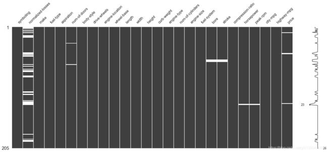
# missing values in normalied-losses
print(data[pd.isnull(data['normalized-losses'])].shape)
data[pd.isnull(data['normalized-losses'])].head()
(41, 26)
Out[5]:
| symboling | normalized-losses | make | fuel-type | aspiration | num-of-doors | body-style | drive-wheels | engine-location | wheel-base | ... | engine-size | fuel-system | bore | stroke | compression-ratio | horsepower | peak-rpm | city-mpg | highway-mpg | price | |
|---|---|---|---|---|---|---|---|---|---|---|---|---|---|---|---|---|---|---|---|---|---|
| 0 | 3 | NaN | alfa-romero | gas | std | two | convertible | rwd | front | 88.6 | ... | 130 | mpfi | 3.47 | 2.68 | 9.0 | 111.0 | 5000.0 | 21 | 27 | 13495.0 |
| 1 | 3 | NaN | alfa-romero | gas | std | two | convertible | rwd | front | 88.6 | ... | 130 | mpfi | 3.47 | 2.68 | 9.0 | 111.0 | 5000.0 | 21 | 27 | 16500.0 |
| 2 | 1 | NaN | alfa-romero | gas | std | two | hatchback | rwd | front | 94.5 | ... | 152 | mpfi | 2.68 | 3.47 | 9.0 | 154.0 | 5000.0 | 19 | 26 | 16500.0 |
| 5 | 2 | NaN | audi | gas | std | two | sedan | fwd | front | 99.8 | ... | 136 | mpfi | 3.19 | 3.40 | 8.5 | 110.0 | 5500.0 | 19 | 25 | 15250.0 |
| 7 | 1 | NaN | audi | gas | std | four | wagon | fwd | front | 105.8 | ... | 136 | mpfi | 3.19 | 3.40 | 8.5 | 110.0 | 5500.0 | 19 | 25 | 18920.0 |
5 rows × 26 columns
sns.set(style = "ticks")
plt.figure(figsize = (12, 5))
c = '#366DE8'
# ECDF经验累积分布函数,用样本推断总体的状态,性质与概率分布函数一致
plt.subplot(121)
cdf = ECDF(data['normalized-losses'])
plt.plot(cdf.x, cdf.y, label = "statmodels", color = c);
plt.xlabel('normalized losses'); plt.ylabel('ECDF');

# overall distribution
plt.subplot(122)
#dropna()为滤除缺失数据
#bins为蓝箱子的个数
plt.hist(data['normalized-losses'].dropna(),
         bins = int(np.sqrt(len(data['normalized-losses']))),
         color = c);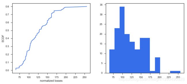
可以发现 80% 的 normalized losses 是低于200 并且绝大多数低于125.
一个基本的想法就是用中位数来进行填充,但是我们得来想一想,这个特征跟哪些因素可能有关呢?应该是保险的情况吧,所以我们可以分组来进行填充这样会更精确一些。
首先来看一下对于不同保险情况的统计指标:
#以symboling对normalized-losses进行分类
data.groupby('symboling')['normalized-losses'].describe()
| count | mean | std | min | 25% | 50% | 75% | max | |
|---|---|---|---|---|---|---|---|---|
| symboling | ||||||||
| -2 | 3.0 | 103.000000 | 0.000000 | 103.0 | 103.00 | 103.0 | 103.0 | 103.0 |
| -1 | 20.0 | 85.600000 | 18.528499 | 65.0 | 71.75 | 91.5 | 95.0 | 137.0 |
| 0 | 48.0 | 113.166667 | 32.510773 | 77.0 | 91.00 | 102.0 | 120.5 | 192.0 |
| 1 | 47.0 | 128.574468 | 28.478630 | 74.0 | 105.50 | 125.0 | 148.0 | 231.0 |
| 2 | 29.0 | 125.689655 | 30.167513 | 83.0 | 94.00 | 134.0 | 137.0 | 192.0 |
| 3 | 17.0 | 168.647059 | 30.636867 | 142.0 | 150.00 | 150.0 | 194.0 | 256.0 |
# replacing
#因为其他维度的缺失数据较少,因此滤除其他维度的缺失数据,丢弃所有带NaN的行。单就normalized-losses一种缺失数据记性填充。
#按保險風險等級分組得到平均值並對normalized-losses列的缺失值進行填充
data = data.dropna(subset = ['price', 'bore', 'stroke', 'peak-rpm', 'horsepower', 'num-of-doors'])
data['normalized-losses'] = data.groupby('symboling')['normalized-losses'].transform(lambda x: x.fillna(x.mean()))

print('In total:', data.shape)
data.head()
In total: (193, 26)
Out[8]:
| symboling | normalized-losses | make | fuel-type | aspiration | num-of-doors | body-style | drive-wheels | engine-location | wheel-base | ... | engine-size | fuel-system | bore | stroke | compression-ratio | horsepower | peak-rpm | city-mpg | highway-mpg | price | |
|---|---|---|---|---|---|---|---|---|---|---|---|---|---|---|---|---|---|---|---|---|---|
| 0 | 3 | 174.384615 | alfa-romero | gas | std | two | convertible | rwd | front | 88.6 | ... | 130 | mpfi | 3.47 | 2.68 | 9.0 | 111.0 | 5000.0 | 21 | 27 | 13495.0 |
| 1 | 3 | 174.384615 | alfa-romero | gas | std | two | convertible | rwd | front | 88.6 | ... | 130 | mpfi | 3.47 | 2.68 | 9.0 | 111.0 | 5000.0 | 21 | 27 | 16500.0 |
| 2 | 1 | 128.152174 | alfa-romero | gas | std | two | hatchback | rwd | front | 94.5 | ... | 152 | mpfi | 2.68 | 3.47 | 9.0 | 154.0 | 5000.0 | 19 | 26 | 16500.0 |
| 3 | 2 | 164.000000 | audi | gas | std | four | sedan | fwd | front | 99.8 | ... | 109 | mpfi | 3.19 | 3.40 | 10.0 | 102.0 | 5500.0 | 24 | 30 | 13950.0 |
| 4 | 2 | 164.000000 | audi | gas | std | four | sedan | 4wd | front | 99.4 | ... | 136 | mpfi | 3.19 | 3.40 | 8.0 | 115.0 | 5500.0 | 18 | 22 | 17450.0 |
5 rows × 26 columns
特征相关性
#计算列与列之间的相关系数,越趋近1相关性越强。
#缺失值處理後,我們還需要分析特徵之間存在的相關性,如果相關性趨向於1,說明這兩個特徵是一回事,可以去掉其中一個特徵,避免出現多重共線。
#整个矩阵数据以对角线成对称排列,因此只保留一半数据即可,同时对角线为1,表示自己和自己,没有分析意义,因此置0
cormatrix = data.corr()#corr:得到相關矩陣,每個值是各個列的相關係數,如:symboling與normalized-losses列的相關係數是0.593658。
cormatrix
| symboling | normalized-losses | wheel-base | length | width | height | curb-weight | engine-size | bore | stroke | compression-ratio | horsepower | peak-rpm | city-mpg | highway-mpg | price | |
|---|---|---|---|---|---|---|---|---|---|---|---|---|---|---|---|---|
| symboling | 1.000000 | 0.593658 | -0.536516 | -0.363194 | -0.247741 | -0.517803 | -0.231086 | -0.068327 | -0.144785 | -0.010884 | -0.175160 | 0.069491 | 0.227899 | 0.017639 | 0.085775 | -0.084835 |
| normalized-losses | 0.593658 | 1.000000 | -0.167286 | -0.038857 | 0.034178 | -0.445925 | 0.085758 | 0.152544 | 0.032765 | 0.057834 | -0.149620 | 0.277376 | 0.245497 | -0.245313 | -0.189911 | 0.160602 |
| wheel-base | -0.536516 | -0.167286 | 1.000000 | 0.879307 | 0.818465 | 0.591239 | 0.782173 | 0.568375 | 0.495957 | 0.174225 | 0.252234 | 0.377040 | -0.350823 | -0.504499 | -0.571771 | 0.584951 |
| length | -0.363194 | -0.038857 | 0.879307 | 1.000000 | 0.857368 | 0.491050 | 0.882694 | 0.686998 | 0.606373 | 0.121888 | 0.156061 | 0.589650 | -0.276144 | -0.702143 | -0.731264 | 0.695928 |
| width | -0.247741 | 0.034178 | 0.818465 | 0.857368 | 1.000000 | 0.310640 | 0.867640 | 0.739903 | 0.541633 | 0.188733 | 0.188631 | 0.621532 | -0.247612 | -0.657153 | -0.702009 | 0.754649 |
| height | -0.517803 | -0.445925 | 0.591239 | 0.491050 | 0.310640 | 1.000000 | 0.305837 | 0.026906 | 0.182445 | -0.054338 | 0.253934 | -0.081730 | -0.257334 | -0.111166 | -0.159850 | 0.136234 |
| curb-weight | -0.231086 | 0.085758 | 0.782173 | 0.882694 | 0.867640 | 0.305837 | 1.000000 | 0.857188 | 0.645070 | 0.175349 | 0.161030 | 0.762154 | -0.278528 | -0.777763 | -0.818104 | 0.835368 |
| engine-size | -0.068327 | 0.152544 | 0.568375 | 0.686998 | 0.739903 | 0.026906 | 0.857188 | 1.000000 | 0.581854 | 0.214518 | 0.025257 | 0.845325 | -0.217769 | -0.716378 | -0.737531 | 0.888778 |
| bore | -0.144785 | 0.032765 | 0.495957 | 0.606373 | 0.541633 | 0.182445 | 0.645070 | 0.581854 | 1.000000 | -0.065038 | -0.004172 | 0.572972 | -0.273766 | -0.601369 | -0.608804 | 0.546295 |
| stroke | -0.010884 | 0.057834 | 0.174225 | 0.121888 | 0.188733 | -0.054338 | 0.175349 | 0.214518 | -0.065038 | 1.000000 | 0.199600 | 0.102913 | -0.068420 | -0.031248 | -0.040274 | 0.096007 |
| compression-ratio | -0.175160 | -0.149620 | 0.252234 | 0.156061 | 0.188631 | 0.253934 | 0.161030 | 0.025257 | -0.004172 | 0.199600 | 1.000000 | -0.203818 | -0.439741 | 0.314648 | 0.249669 | 0.074483 |
| horsepower | 0.069491 | 0.277376 | 0.377040 | 0.589650 | 0.621532 | -0.081730 | 0.762154 | 0.845325 | 0.572972 | 0.102913 | -0.203818 | 1.000000 | 0.101383 | -0.833615 | -0.812078 | 0.812453 |
| peak-rpm | 0.227899 | 0.245497 | -0.350823 | -0.276144 | -0.247612 | -0.257334 | -0.278528 | -0.217769 | -0.273766 | -0.068420 | -0.439741 | 0.101383 | 1.000000 | -0.061032 | -0.008412 | -0.103835 |
| city-mpg | 0.017639 | -0.245313 | -0.504499 | -0.702143 | -0.657153 | -0.111166 | -0.777763 | -0.716378 | -0.601369 | -0.031248 | 0.314648 | -0.833615 | -0.061032 | 1.000000 | 0.971975 | -0.706618 |
| highway-mpg | 0.085775 | -0.189911 | -0.571771 | -0.731264 | -0.702009 | -0.159850 | -0.818104 | -0.737531 | -0.608804 | -0.040274 | 0.249669 | -0.812078 | -0.008412 | 0.971975 | 1.000000 | -0.719178 |
| price | -0.084835 | 0.160602 | 0.584951 | 0.695928 | 0.754649 | 0.136234 | 0.835368 | 0.888778 | 0.546295 | 0.096007 | 0.074483 | 0.812453 | -0.103835 | -0.706618 | -0.719178 | 1.000000 |
#返回函数的上三角矩阵,把对角线上的置0,让他们不是最高的。
#np.tri()生成下三角矩阵,k=-1即对角线向下偏移一个单位,对角线及以上元素全都置零
#.T矩阵转置,下三角矩阵转置变成上三角矩阵
cormatrix *= np.tri(*cormatrix.values.shape, k=-1).T
cormatrix| symboling | normalized-losses | wheel-base | length | width | height | curb-weight | engine-size | bore | stroke | compression-ratio | horsepower | peak-rpm | city-mpg | highway-mpg | price | |
|---|---|---|---|---|---|---|---|---|---|---|---|---|---|---|---|---|
| symboling | 0.0 | 0.593658 | -0.536516 | -0.363194 | -0.247741 | -0.517803 | -0.231086 | -0.068327 | -0.144785 | -0.010884 | -0.175160 | 0.069491 | 0.227899 | 0.017639 | 0.085775 | -0.084835 |
| normalized-losses | 0.0 | 0.000000 | -0.167286 | -0.038857 | 0.034178 | -0.445925 | 0.085758 | 0.152544 | 0.032765 | 0.057834 | -0.149620 | 0.277376 | 0.245497 | -0.245313 | -0.189911 | 0.160602 |
| wheel-base | -0.0 | -0.000000 | 0.000000 | 0.879307 | 0.818465 | 0.591239 | 0.782173 | 0.568375 | 0.495957 | 0.174225 | 0.252234 | 0.377040 | -0.350823 | -0.504499 | -0.571771 | 0.584951 |
| length | -0.0 | -0.000000 | 0.000000 | 0.000000 | 0.857368 | 0.491050 | 0.882694 | 0.686998 | 0.606373 | 0.121888 | 0.156061 | 0.589650 | -0.276144 | -0.702143 | -0.731264 | 0.695928 |
| width | -0.0 | 0.000000 | 0.000000 | 0.000000 | 0.000000 | 0.310640 | 0.867640 | 0.739903 | 0.541633 | 0.188733 | 0.188631 | 0.621532 | -0.247612 | -0.657153 | -0.702009 | 0.754649 |
| height | -0.0 | -0.000000 | 0.000000 | 0.000000 | 0.000000 | 0.000000 | 0.305837 | 0.026906 | 0.182445 | -0.054338 | 0.253934 | -0.081730 | -0.257334 | -0.111166 | -0.159850 | 0.136234 |
| curb-weight | -0.0 | 0.000000 | 0.000000 | 0.000000 | 0.000000 | 0.000000 | 0.000000 | 0.857188 | 0.645070 | 0.175349 | 0.161030 | 0.762154 | -0.278528 | -0.777763 | -0.818104 | 0.835368 |
| engine-size | -0.0 | 0.000000 | 0.000000 | 0.000000 | 0.000000 | 0.000000 | 0.000000 | 0.000000 | 0.581854 | 0.214518 | 0.025257 | 0.845325 | -0.217769 | -0.716378 | -0.737531 | 0.888778 |
| bore | -0.0 | 0.000000 | 0.000000 | 0.000000 | 0.000000 | 0.000000 | 0.000000 | 0.000000 | 0.000000 | -0.065038 | -0.004172 | 0.572972 | -0.273766 | -0.601369 | -0.608804 | 0.546295 |
| stroke | -0.0 | 0.000000 | 0.000000 | 0.000000 | 0.000000 | -0.000000 | 0.000000 | 0.000000 | -0.000000 | 0.000000 | 0.199600 | 0.102913 | -0.068420 | -0.031248 | -0.040274 | 0.096007 |
| compression-ratio | -0.0 | -0.000000 | 0.000000 | 0.000000 | 0.000000 | 0.000000 | 0.000000 | 0.000000 | -0.000000 | 0.000000 | 0.000000 | -0.203818 | -0.439741 | 0.314648 | 0.249669 | 0.074483 |
| horsepower | 0.0 | 0.000000 | 0.000000 | 0.000000 | 0.000000 | -0.000000 | 0.000000 | 0.000000 | 0.000000 | 0.000000 | -0.000000 | 0.000000 | 0.101383 | -0.833615 | -0.812078 | 0.812453 |
| peak-rpm | 0.0 | 0.000000 | -0.000000 | -0.000000 | -0.000000 | -0.000000 | -0.000000 | -0.000000 | -0.000000 | -0.000000 | -0.000000 | 0.000000 | 0.000000 | -0.061032 | -0.008412 | -0.103835 |
| city-mpg | 0.0 | -0.000000 | -0.000000 | -0.000000 | -0.000000 | -0.000000 | -0.000000 | -0.000000 | -0.000000 | -0.000000 | 0.000000 | -0.000000 | -0.000000 | 0.000000 | 0.971975 | -0.706618 |
| highway-mpg | 0.0 | -0.000000 | -0.000000 | -0.000000 | -0.000000 | -0.000000 | -0.000000 | -0.000000 | -0.000000 | -0.000000 | 0.000000 | -0.000000 | -0.000000 | 0.000000 | 0.000000 | -0.719178 |
| price | -0.0 | 0.000000 | 0.000000 | 0.000000 | 0.000000 | 0.000000 | 0.000000 | 0.000000 | 0.000000 | 0.000000 | 0.000000 | 0.000000 | -0.000000 | -0.000000 | -0.000000 | 0.000000 |
cormatrix = cormatrix.stack()#在用pandas進行數據重排時,經常用到stack和unstack兩個函數。stack:以列爲索引堆積,unstack:以行爲索引展開。
cormatrix
#返回某个变量和其他变量的相关性
symboling          symboling            0.000000
                   normalized-losses    0.593658
                   wheel-base          -0.536516
                   length              -0.363194
                   width               -0.247741
                   height              -0.517803
                   curb-weight         -0.231086
                   engine-size         -0.068327
                   bore                -0.144785
                   stroke              -0.010884
                   compression-ratio   -0.175160
                   horsepower           0.069491
                   peak-rpm             0.227899
                   city-mpg             0.017639
                   highway-mpg          0.085775
                   price               -0.084835
normalized-losses  symboling            0.000000
                   normalized-losses    0.000000
                   wheel-base          -0.167286
                   length              -0.038857
                   width                0.034178
                   height              -0.445925
                   curb-weight          0.085758
                   engine-size          0.152544
                   bore                 0.032765
                   stroke               0.057834
                   compression-ratio   -0.149620
                   horsepower           0.277376
                   peak-rpm             0.245497
                   city-mpg            -0.245313
                                          ...
highway-mpg        wheel-base          -0.000000
                   length              -0.000000
                   width               -0.000000
                   height              -0.000000
                   curb-weight         -0.000000
                   engine-size         -0.000000
                   bore                -0.000000
                   stroke              -0.000000
                   compression-ratio    0.000000
                   horsepower          -0.000000
                   peak-rpm            -0.000000
                   city-mpg             0.000000
                   highway-mpg          0.000000
                   price               -0.719178
price              symboling           -0.000000
                   normalized-losses    0.000000
                   wheel-base           0.000000
                   length               0.000000
                   width                0.000000
                   height               0.000000
                   curb-weight          0.000000
                   engine-size          0.000000
                   bore                 0.000000
                   stroke               0.000000
                   compression-ratio    0.000000
                   horsepower           0.000000
                   peak-rpm            -0.000000
                   city-mpg            -0.000000
                   highway-mpg         -0.000000
                   price                0.000000
Length: 256, dtype: float64
#reindex(新索引):按新索引排序;
#abs():返回絕對值;
#sort_values():排序,ascending=False:升序,默認true:升序;
#reset_index():將行索引轉爲新列的值,並命名level_
#When we reset the index, the old index is added as a column, and a new sequential index is used:
cormatrix = cormatrix.reindex(cormatrix.abs().sort_values(ascending=False).index).reset_index()
cormatrix.columns = ["FirstVariable", "SecondVariable", "Correlation"]
cormatrix.head(10)
#除此我們還需要分析特徵之間是否存在一些邏輯關係,比如:數據中有長、寬、高三個特徵,我們可以將其合併相乘得一個體積變量。
#如第一个数据是0.97,意味着两个变量过于相似,没什么区别,二者选其一就可以了
	FirstVariable	SecondVariable	Correlation
0	city-mpg	highway-mpg	0.971975
1	engine-size	price	0.888778
2	length	curb-weight	0.882694
3	wheel-base	length	0.879307
4	width	curb-weight	0.867640
5	length	width	0.857368
6	curb-weight	engine-size	0.857188
7	engine-size	horsepower	0.845325
8	curb-weight	price	0.835368
9	horsepower	city-mpg	-0.833615
city_mpg 和 highway-mpg 这哥俩差不多是一个意思了. 对于这个长宽高,他们应该存在某种配对关系,给他们合体吧!
data['volume'] = data.length * data.width * data.height
#drop默认删除行元素,删除列需加 axis = 1
data.drop(['width', 'length', 'height',
           'curb-weight', 'city-mpg'],
          axis = 1, # 1 for columns
          inplace = True)
# new variables
data.columns
Index(['symboling', 'normalized-losses', 'make', 'fuel-type', 'aspiration',
       'num-of-doors', 'body-style', 'drive-wheels', 'engine-location',
       'wheel-base', 'engine-type', 'num-of-cylinders', 'engine-size',
       'fuel-system', 'bore', 'stroke', 'compression-ratio', 'horsepower',
       'peak-rpm', 'highway-mpg', 'price', 'volume'],
      dtype='object')
# Compute the correlation matrix
corr_all = data.corr()

# Generate a mask for the upper triangle
#构造一个蒙版布尔型,同corr_all一致的零矩阵,然后从中取上三角矩阵。去下三角矩阵是np.tril_indices_from(mask)
#其目的是剔除冗余映射,只取一半就好
mask = np.zeros_like(corr_all, dtype = np.bool)
mask[np.triu_indices_from(mask)] = True

# Set up the matplotlib figure
#plt.subplots() 返回一个 Figure实例fig 和一个 AxesSubplot实例ax 。这个很好理解,fig代表整个图像,ax代表坐标轴和画的图。
f, ax = plt.subplots(figsize = (11, 9))

# Draw the heatmap with the mask and correct aspect ratio
#mask=True ,上三角单元将自动被屏蔽
sns.heatmap(corr_all, mask = mask,
            square = True, linewidths = .5, ax = ax, cmap = "YlOrRd")
plt.show() 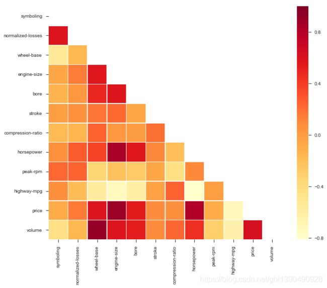
看起来 price 跟这几个的相关程度比较大 wheel-base,enginine-size, bore,horsepower.
#多变量图,对角线为分布直方图。hue为指定变量
sns.pairplot(data, hue = 'fuel-type', palette = 'husl',markers=["o", "s"])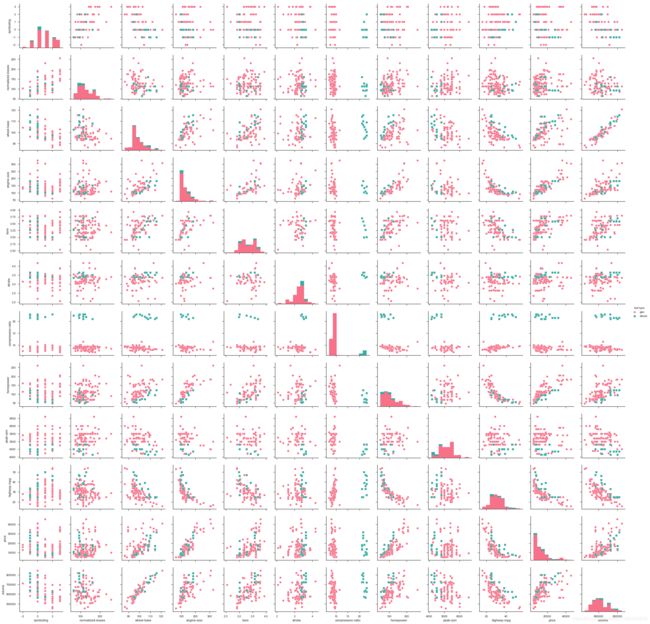
让我们仔细看看价格和马力变量之间的关系
#绘制线性回归
sns.lmplot('price', 'horsepower', data,
           hue = 'fuel-type', col = 'fuel-type',  row = 'num-of-doors',
           palette = 'plasma',
           fit_reg = True);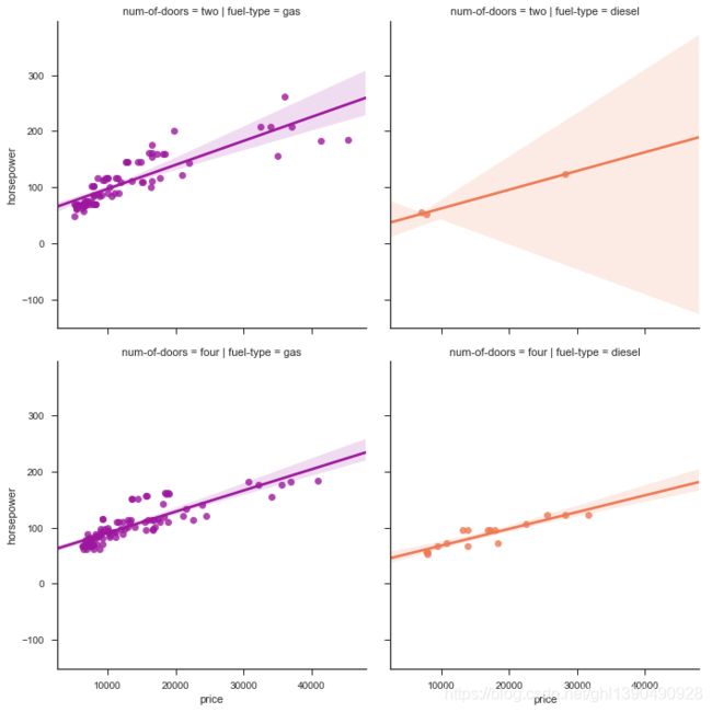
事实上,对于燃料的类型和数门变量,我们看到,在一辆汽车马力的增加与价格成比例的增加相关的各个层面
预处理
如果一个特性的方差比其他的要大得多,那么它可能支配目标函数,使估计者不能像预期的那样正确地从其他特性中学习。这就是为什么我们需要首先对数据进行缩放。
对连续值进行标准化(或归一化)
# 选定目标变量
target = data.price
# 得到剔除掉目标变量的其他变量名
regressors = [x for x in data.columns if x not in ['price']]
#.loc[],中括号里面是先行后列,以逗号分割,行和列分别是行标签和列标签, 通过.loc[]定位到某行某列
features = data.loc[:, regressors]
#筛选出数据类型不是字符型的列
num = ['symboling', 'normalized-losses', 'volume', 'horsepower', 'wheel-base',
       'bore', 'stroke','compression-ratio', 'peak-rpm']

# scale the data,StandardScaler()库可保存训练集中的均值、方差参数,然后直接用于转换测试集数据
standard_scaler = StandardScaler()
#进行标准化处理
features[num] = standard_scaler.fit_transform(features[num])

# glimpse
features.head()
| symboling | normalized-losses | make | fuel-type | aspiration | num-of-doors | body-style | drive-wheels | engine-location | wheel-base | ... | num-of-cylinders | engine-size | fuel-system | bore | stroke | compression-ratio | horsepower | peak-rpm | highway-mpg | volume | |
|---|---|---|---|---|---|---|---|---|---|---|---|---|---|---|---|---|---|---|---|---|---|
| 0 | 1.78685 | 1.477685 | alfa-romero | gas | std | two | convertible | rwd | front | -1.682379 | ... | four | 130 | mpfi | 0.513027 | -1.808186 | -0.288273 | 0.198569 | -0.213359 | 27 | -1.168294 |
| 1 | 1.78685 | 1.477685 | alfa-romero | gas | std | two | convertible | rwd | front | -1.682379 | ... | four | 130 | mpfi | 0.513027 | -1.808186 | -0.288273 | 0.198569 | -0.213359 | 27 | -1.168294 |
| 2 | 0.16397 | 0.144710 | alfa-romero | gas | std | two | hatchback | rwd | front | -0.720911 | ... | six | 152 | mpfi | -2.394827 | 0.702918 | -0.288273 | 1.334283 | -0.213359 | 26 | -0.422041 |
| 3 | 0.97541 | 1.178276 | audi | gas | std | four | sedan | fwd | front | 0.142781 | ... | four | 109 | mpfi | -0.517605 | 0.480415 | -0.036204 | -0.039139 | 0.856208 | 30 | 0.169527 |
| 4 | 0.97541 | 1.178276 | audi | gas | std | four | sedan | 4wd | front | 0.077596 | ... | five | 136 | mpfi | -0.517605 | 0.480415 | -0.540341 | 0.304217 | 0.856208 | 22 | 0.193551 |
5 rows × 21 columns
对分类属性就行one-hot编码
# 筛选出分类变量列名
classes = ['make', 'fuel-type', 'aspiration', 'num-of-doors',
           'body-style', 'drive-wheels', 'engine-location',
           'engine-type', 'num-of-cylinders', 'fuel-system']

# 将数据转化成独热编码, 即對非數值類型的字符進行分類轉換成數字。用0-1表示,这就将许多指标划分成若干子列,因此现在总共是66列
dummies = pd.get_dummies(features[classes])
#将分类处理后的数据列添加进列表中同时删除处理前的列
features = features.join(dummies).drop(classes,
                                       axis = 1)

# new dataset
print('In total:', features.shape)
features.head()| symboling | normalized-losses | wheel-base | engine-size | bore | stroke | compression-ratio | horsepower | peak-rpm | highway-mpg | ... | num-of-cylinders_six | num-of-cylinders_three | num-of-cylinders_twelve | fuel-system_1bbl | fuel-system_2bbl | fuel-system_idi | fuel-system_mfi | fuel-system_mpfi | fuel-system_spdi | fuel-system_spfi | |
|---|---|---|---|---|---|---|---|---|---|---|---|---|---|---|---|---|---|---|---|---|---|
| 0 | 1.78685 | 1.477685 | -1.682379 | 130 | 0.513027 | -1.808186 | -0.288273 | 0.198569 | -0.213359 | 27 | ... | 0 | 0 | 0 | 0 | 0 | 0 | 0 | 1 | 0 | 0 |
| 1 | 1.78685 | 1.477685 | -1.682379 | 130 | 0.513027 | -1.808186 | -0.288273 | 0.198569 | -0.213359 | 27 | ... | 0 | 0 | 0 | 0 | 0 | 0 | 0 | 1 | 0 | 0 |
| 2 | 0.16397 | 0.144710 | -0.720911 | 152 | -2.394827 | 0.702918 | -0.288273 | 1.334283 | -0.213359 | 26 | ... | 1 | 0 | 0 | 0 | 0 | 0 | 0 | 1 | 0 | 0 |
| 3 | 0.97541 | 1.178276 | 0.142781 | 109 | -0.517605 | 0.480415 | -0.036204 | -0.039139 | 0.856208 | 30 | ... | 0 | 0 | 0 | 0 | 0 | 0 | 0 | 1 | 0 | 0 |
| 4 | 0.97541 | 1.178276 | 0.077596 | 136 | -0.517605 | 0.480415 | -0.540341 | 0.304217 | 0.856208 | 22 | ... | 0 | 0 | 0 | 0 | 0 | 0 | 0 | 1 | 0 | 0 |
5 rows × 66 columns
划分数据集】
# sklearn.model_selection.train_test_split随机划分训练集和测试集
X_train, X_test, y_train, y_test = train_test_split(features, target,
                                                    test_size = 0.3,
                                                    random_state = seed)
print("Train", X_train.shape, "and test", X_test.shape)
X_train.head()
Train (135, 66) and test (58, 66)
Out[30]:
| symboling | normalized-losses | wheel-base | engine-size | bore | stroke | compression-ratio | horsepower | peak-rpm | highway-mpg | ... | num-of-cylinders_six | num-of-cylinders_three | num-of-cylinders_twelve | fuel-system_1bbl | fuel-system_2bbl | fuel-system_idi | fuel-system_mfi | fuel-system_mpfi | fuel-system_spdi | fuel-system_spfi | |
|---|---|---|---|---|---|---|---|---|---|---|---|---|---|---|---|---|---|---|---|---|---|
| 196 | -2.270351 | -0.580478 | 0.876104 | 141 | 1.654084 | -0.314238 | -0.162238 | 0.277805 | 0.642295 | 28 | ... | 0 | 0 | 0 | 0 | 0 | 0 | 0 | 1 | 0 | 0 |
| 190 | 1.786850 | 3.830822 | -0.720911 | 109 | -0.517605 | 0.480415 | -0.414307 | -0.356082 | 0.856208 | 29 | ... | 0 | 0 | 0 | 0 | 0 | 0 | 0 | 1 | 0 | 0 |
| 133 | 0.975410 | -0.551646 | 0.028708 | 121 | 0.770685 | -0.568527 | -0.212652 | 0.172157 | 0.321425 | 28 | ... | 0 | 0 | 0 | 0 | 0 | 0 | 0 | 1 | 0 | 0 |
| 180 | -1.458911 | -0.955294 | 0.908696 | 171 | -0.223138 | 0.321485 | -0.237859 | 1.387107 | 0.214468 | 24 | ... | 1 | 0 | 0 | 0 | 0 | 0 | 0 | 1 | 0 | 0 |
| 38 | -0.647470 | -0.493982 | -0.394990 | 110 | -0.664838 | 1.052565 | -0.288273 | -0.461730 | 1.497949 | 33 | ... | 0 | 0 | 0 | 1 | 0 | 0 | 0 | 0 | 0 | 0 |
5 rows × 66 columns
Lasso回归
多加了一個絕對值項來懲罰過大的係數((預測值Y-實際值Y)/N-入|w|),alphas參數即是入,懲罰力度越大,alphas值越大,若alphas=0,即沒有懲罰項,就等於線性迴歸,最小二乘法。
# logarithmic scale: log base 2
# high values to zero-out more variables
#選擇alphas值的方法有兩個:
#方法一:建一個for循環,測試alphas等於多少時方程最優
alphas = 2. ** np.arange(2, 12) #array([2,3,4,5,6,7,8,9,10,11])
scores = np.empty_like(alphas)
#用不同的alphas值做模型
#enumerate() 函數用於將一個可遍歷的數據對象(如列表、元組或字符串)組合爲一個索引序列,同時列出數據和數據下標,一般用在 for 循環當中
for i, a in enumerate(alphas): #i:alphas索引序列,a:alphas數據
lasso = Lasso(random_state = seed) #指定lasso模型
lasso.set_params(alpha = a) #確定alpha值
lasso.fit(X_train, y_train) #.fit(x,y) 執行
scores[i] = lasso.score(X_test, y_test) #用測試值測算公式
#方法二:常用交叉驗證
#lassocv:交叉驗證模型,cv:交叉驗證切分個數
#lassocv返回拟合优度这一统计学指标,越趋近1,拟合程度越好
lassocv = LassoCV(cv = 10, random_state = seed)#制定模型,将训练集平均切10分,9份用来做训练,1份用来做验证,可设置alphas=[]是多少(序列格式),默认不设置则找适合训练集最优alpha
lassocv.fit(features, target) #输入数据训练训练模型
lassocv_score = lassocv.score(features, target) #测试模型,返回r^2
lassocv_alpha = lassocv.alpha_ #即确定出最佳惩罚系数 入
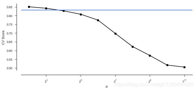
plt.figure(figsize = (10, 4))
plt.plot(alphas, scores, '-ko')
#在图上添加一条水平线
plt.axhline(lassocv_score, color = c)
plt.xlabel(r'$\alpha$')
plt.ylabel('CV Score')
plt.xscale('log', basex = 2)
#两个坐标轴与图像的偏移距离
sns.despine(offset = 15)
print('CV results:', lassocv_score, lassocv_alpha)CV results: 0.8319664321686158 342.0081418966275
# lassocv 回归系数   lassocv.coef_是参数向量w
#pd.Series(data,index)
coefs = pd.Series(lassocv.coef_, index = features.columns)  # .coef_ 可以返回经过学习后的所有 feature 的参数。

# prints out the number of picked/eliminated features
print("Lasso picked " + str(sum(coefs != 0)) + " features and eliminated the other " +  \
      str(sum(coefs == 0)) + " features.")
#在汽车价格预测中,最重要的正向 feature 是 volume,这个比较贴近现实
# takes first and last 10
coefs = pd.concat([coefs.sort_values().head(5), coefs.sort_values().tail(5)])   #将相同字段首尾相接

plt.figure(figsize = (10, 4))
coefs.plot(kind = "barh", color = c)
plt.title("Coefficients in the Lasso Model")
plt.show() 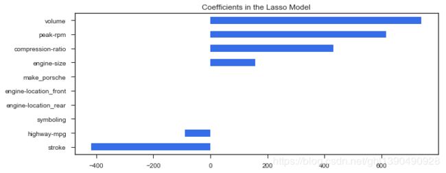
model_l1 = LassoCV(alphas = alphas, cv = 10, random_state = seed).fit(X_train, y_train)
y_pred_l1 = model_l1.predict(X_test)

model_l1.score(X_test, y_test)
0.8277858219151173
# residual plot
plt.rcParams['figure.figsize'] = (6.0, 6.0)

preds = pd.DataFrame({"preds": model_l1.predict(X_train), "true": y_train})
preds["residuals"] = preds["true"] - preds["preds"]
preds.plot(x = "preds", y = "residuals", kind = "scatter", color = c) 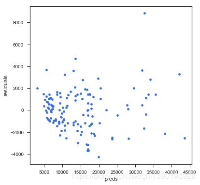
def MSE(y_true,y_pred):
    mse = mean_squared_error(y_true, y_pred)
    print('MSE: %2.3f' % mse)
    return mse

def R2(y_true,y_pred):
    r2 = r2_score(y_true, y_pred)
    print('R2: %2.3f' % r2)
    return r2

MSE(y_test, y_pred_l1); R2(y_test, y_pred_l1);
MSE: 3993172.564
R2: 0.828
# predictions
d = {'true' : list(y_test),
     'predicted' : pd.Series(y_pred_l1)
    }

pd.DataFrame(d).head()| predicted | true | |
|---|---|---|
| 0 | 8503.836069 | 8499.0 |
| 1 | 17137.224283 | 17450.0 |
| 2 | 8511.911025 | 9279.0 |
| 3 | 10935.968247 | 7975.0 |
| 4 | 6233.718975 | 6692.0 |