【活动打卡】【Datawhale】第16期 机器学习算法梳理（AI入门体验） Task01：基于逻辑回归的分类预测

1.逻辑回归原理简介

当 z≥0 时,y≥0.5,分类为1，当 z<0 时,y<0.5,分类为0，其对应的y值我们可以视为类别1的概率预测值。Logistic回归虽然名字里带“回归”，但是它实际上是一种分类方法，主要用于两分类问题（即输出只有两种，分别代表两个类别），所以利用了Logistic函数（或称为Sigmoid函数），函数形式为：

$$logi(z)=\frac{1}{1+e^{-z}}$$

对应的函数图像可以表示如下:

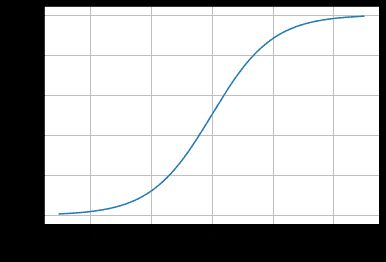
通过上图我们可以发现 Logistic 函数是单调递增函数，并且在z=0处分界，而回归的基本方程为

$$p=p(y=1|x,\theta )=h_{\theta }(x,\theta )=\frac{1}{1+e^{-(w_0+{\sum }_i^N{w}_i{x}_i)}}$$

将回归方程代入其中为：

$$p=p(y=1|x,\theta )=h_{\theta }(x,\theta )，p(y=0|x,\theta )=1-h_{\theta }(x,\theta )$$

所以，逻辑回归从其原理上来说，逻辑回归其实是实现了一个决策边界：对于函数 $y=\frac{1}{1+e^{-z}}$ ，当 z≥0 时,y≥0.5,分类为1，当 z<0 时,y<0.5,分类为0，其对应的y值我们可以视为类别1的概率预测值。

对于模型的训练而言：实质上来说就是利用数据求解出对应的模型的特定的ω。从而得到一个针对于当前数据的特征逻辑回归模型。而对于多分类而言，将多个二分类的逻辑回归组合，即可实现多分类。

2.Demo实践

scikit-learn 是基于 Python 语言的机器学习工具，逻辑回归在 sklearn 中是用 sklearn.linear_model 中的 LogisticRegression 实现。

Step1：库函数导入

##  基础函数库
import numpy as np 

## 导入画图库
import matplotlib.pyplot as plt
import seaborn as sns

## 导入逻辑回归模型函数
from sklearn.linear_model import LogisticRegression

Step2：训练模型

##Demo演示LogisticRegression分类

## 构造数据集
x_fearures = np.array([[-1, -2], [-2, -1], [-3, -2], [1, 3], [2, 1], [3, 2]])
y_label = np.array([0, 0, 0, 1, 1, 1])

## 调用逻辑回归模型
lr_clf = LogisticRegression()

## 用逻辑回归模型拟合构造的数据集
lr_clf = lr_clf.fit(x_fearures, y_label) #其拟合方程为 y=w0+w1*x1+w2*x2

Step3：模型参数查看

##查看其对应模型的w
print('the weight of Logistic Regression:',lr_clf.coef_)
##查看其对应模型的w0
print('the intercept(w0) of Logistic Regression:',lr_clf.intercept_)

the weight of Logistic Regression: [[ 0.73462087 0.6947908 ]]
the intercept(w0) of Logistic Regression: [-0.03643213]

Step4：数据和模型可视化

## 可视化构造的数据样本点
plt.figure()
plt.scatter(x_fearures[:,0],x_fearures[:,1], c=y_label, s=50, cmap='viridis')
plt.title('Dataset')
plt.show()

# 可视化决策边界
plt.figure()
plt.scatter(x_fearures[:,0],x_fearures[:,1], c=y_label, s=50, cmap='viridis')
plt.title('Dataset')

nx, ny = 200, 100
x_min, x_max = plt.xlim()
y_min, y_max = plt.ylim()
x_grid, y_grid = np.meshgrid(np.linspace(x_min, x_max, nx),np.linspace(y_min, y_max, ny))

z_proba = lr_clf.predict_proba(np.c_[x_grid.ravel(), y_grid.ravel()])
z_proba = z_proba[:, 1].reshape(x_grid.shape)
plt.contour(x_grid, y_grid, z_proba, [0.5], linewidths=2., colors='blue')

plt.show()

### 可视化预测新样本

plt.figure()
## new point 1
x_fearures_new1 = np.array([[0, -1]])
plt.scatter(x_fearures_new1[:,0],x_fearures_new1[:,1], s=50, cmap='viridis')
plt.annotate(s='New point 1',xy=(0,-1),xytext=(-2,0),color='blue',arrowprops=dict(arrowstyle='-|>',connectionstyle='arc3',color='red'))

## new point 2
x_fearures_new2 = np.array([[1, 2]])
plt.scatter(x_fearures_new2[:,0],x_fearures_new2[:,1], s=50, cmap='viridis')
plt.annotate(s='New point 2',xy=(1,2),xytext=(-1.5,2.5),color='red',arrowprops=dict(arrowstyle='-|>',connectionstyle='arc3',color='red'))

## 训练样本
plt.scatter(x_fearures[:,0],x_fearures[:,1], c=y_label, s=50, cmap='viridis')
plt.title('Dataset')

# 可视化决策边界
plt.contour(x_grid, y_grid, z_proba, [0.5], linewidths=2., colors='blue')

plt.show()

Step5：模型预测

##在训练集和测试集上分布利用训练好的模型进行预测
y_label_new1_predict=lr_clf.predict(x_fearures_new1)
y_label_new2_predict=lr_clf.predict(x_fearures_new2)
print('The New point 1 predict class:\n',y_label_new1_predict)
print('The New point 2 predict class:\n',y_label_new2_predict)
##由于逻辑回归模型是概率预测模型,所以我们可以利用predict_proba函数预测其概率
y_label_new1_predict_proba=lr_clf.predict_proba(x_fearures_new1)
y_label_new2_predict_proba=lr_clf.predict_proba(x_fearures_new2)
print('The New point 1 predict Probability of each class:\n',y_label_new1_predict_proba)
print('The New point 2 predict Probability of each class:\n',y_label_new2_predict_proba)

The New point 1 predict class:
[0]
The New point 2 predict class:
[1]
The New point 1 predict Probability of each class:
[[ 0.67507358 0.32492642]]
The New point 2 predict Probability of each class:
[[ 0.11029117 0.88970883]]

可以发现训练好的回归模型将X_new1预测为了类别0（判别面左下侧），X_new2预测为了类别1（判别面右上侧）。其训练得到的逻辑回归模型的概率为0.5的判别面为上图中蓝色的线。

3.基于鸢尾花（iris）数据集的逻辑回归分类实践

鸢尾花（iris）数据集是常用的分类实验数据集，包含150个数据样本，分为3类，每类50个数据，每个数据包含4个属性。可通过花萼长度，花萼宽度，花瓣长度，花瓣宽度4个属性预测鸢尾花卉属于（Setosa，Versicolour，Virginica）三个种类中的哪一类。

Step1：函数库导入

在实践的最开始，我们首先需要导入一些基础的函数库包括：numpy，pandas，matplotlib和seaborn绘图。

##  基础函数库
import numpy as np 
import pandas as pd

## 绘图函数库
import matplotlib.pyplot as plt
import seaborn as sns

Step2：数据读取/载入

然后导入数据集，以下通过表格对变量及其描述做出了解释：

变量	描述
sepal length	花萼长度(cm)
sepal width	花萼宽度(cm)
petal length	花瓣长度(cm)
petal width	花瓣宽度(cm)
target	鸢尾的三个亚属类别,‘setosa’(0), ‘versicolor’(1), ‘virginica’(2)

##我们利用sklearn中自带的iris数据作为数据载入，并利用Pandas转化为DataFrame格式
from sklearn.datasets import load_iris
data = load_iris() #得到数据特征
iris_target = data.target #得到数据对应的标签
iris_features = pd.DataFrame(data=data.data, columns=data.feature_names) #利用Pandas转化为DataFrame格式

Step3：数据信息简单查看

通过一些简单的操作对数据集的信息有一个大概的了解。

##利用.info()查看数据的整体信息
iris_features.info()

RangeIndex: 150 entries, 0 to 149
Data columns (total 4 columns):
sepal length (cm) 150 non-null float64
sepal width (cm) 150 non-null float64
petal length (cm) 150 non-null float64
petal width (cm) 150 non-null float64
dtypes: float64(4)
memory usage: 4.8 KB

##其对应的类别标签为，其中0，1，2分别代表'setosa','versicolor','virginica'三种不同花的类别
iris_target

array([0, 0, 0, 0, 0, 0, 0, 0, 0, 0, 0, 0, 0, 0, 0, 0, 0, 0, 0, 0, 0, 0, 0,
0, 0, 0, 0, 0, 0, 0, 0, 0, 0, 0, 0, 0, 0, 0, 0, 0, 0, 0, 0, 0, 0, 0,
0, 0, 0, 0, 1, 1, 1, 1, 1, 1, 1, 1, 1, 1, 1, 1, 1, 1, 1, 1, 1, 1, 1,
1, 1, 1, 1, 1, 1, 1, 1, 1, 1, 1, 1, 1, 1, 1, 1, 1, 1, 1, 1, 1, 1, 1,
1, 1, 1, 1, 1, 1, 1, 1, 2, 2, 2, 2, 2, 2, 2, 2, 2, 2, 2, 2, 2, 2, 2,
2, 2, 2, 2, 2, 2, 2, 2, 2, 2, 2, 2, 2, 2, 2, 2, 2, 2, 2, 2, 2, 2, 2,
2, 2, 2, 2, 2, 2, 2, 2, 2, 2, 2, 2])

##利用value_counts函数查看每个类别数量
pd.Series(iris_target).value_counts()

2 50
1 50
0 50
dtype: int64

Step4:可视化描述

通过可视化对数据集进一步分析。

## 合并标签和特征信息
iris_all = iris_features.copy() # 进行浅拷贝，防止对于原始数据的修改
iris_all['target'] = iris_target
## 特征与标签组合的散点可视化
sns.pairplot(data=iris_all,diag_kind='hist', hue= 'target')
plt.show()

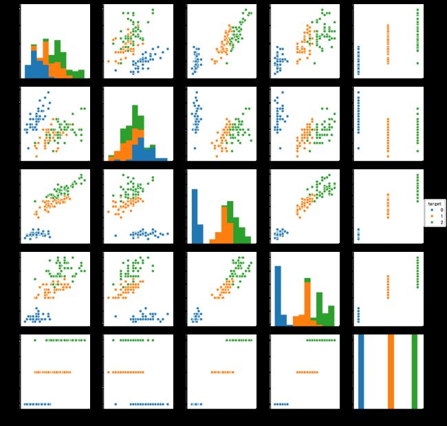
从上图可以发现，在2D情况下不同的特征组合对于不同类别的花的散点分布，以及大概的区分能力。

for col in iris_features.columns:
    sns.boxplot(x='target', y=col, saturation=0.5, palette='pastel', data=iris_all)
    plt.title(col)
    plt.show()

利用箱型图我们也可以得到不同类别在不同特征上的分布差异情况。

# 选取其前三个特征绘制三维散点图
from mpl_toolkits.mplot3d import Axes3D

fig = plt.figure(figsize=(10,8))
ax = fig.add_subplot(111, projection='3d')

iris_all_class0 = iris_all[iris_all['target']==0].values
iris_all_class1 = iris_all[iris_all['target']==1].values
iris_all_class2 = iris_all[iris_all['target']==2].values
# 'setosa'(0), 'versicolor'(1), 'virginica'(2)
ax.scatter(iris_all_class0[:,0], iris_all_class0[:,1], iris_all_class0[:,2],label='setosa')
ax.scatter(iris_all_class1[:,0], iris_all_class1[:,1], iris_all_class1[:,2],label='versicolor')
ax.scatter(iris_all_class2[:,0], iris_all_class2[:,1], iris_all_class2[:,2],label='virginica')
plt.legend()

plt.show()

Step5:利用 逻辑回归模型 在二分类上 进行训练和预测

##为了正确评估模型性能，将数据划分为训练集和测试集，并在训练集上训练模型，在测试集上验证模型性能。
from sklearn.model_selection import train_test_split
##选择其类别为0和1的样本（不包括类别为2的样本）
iris_features_part=iris_features.iloc[:100]
iris_target_part=iris_target[:100]
##测试集大小为20%，80%/20%分
x_train,x_test,y_train,y_test=train_test_split(iris_features_part,iris_target_part,test_size=0.2,random_state=2020)

##从sklearn中导入逻辑回归模型
from sklearn.linear_model import LogisticRegression

##定义逻辑回归模型
clf=LogisticRegression(random_state=0,solver='lbfgs')

##在训练集上训练逻辑回归模型
clf.fit(x_train,y_train)

##查看其对应的w
print('the weight of Logistic Regression:',clf.coef_)

##查看其对应的w0
print('the intercept(w0) of Logistic Regression:',clf.intercept_)

the weight of Logistic Regression: [[ 0.45244919 -0.81010583 2.14700385 0.90450733]]
the intercept(w0) of Logistic Regression: [-6.57504448]

##在训练集和测试集上分布利用训练好的模型进行预测
train_predict=clf.predict(x_train)
test_predict=clf.predict(x_test)

from sklearn import metrics
##利用accuracy（准确度）【预测正确的样本数目占总预测样本数目的比例】评估模型效果
print('The accuracy of the Logistic Regression is:',metrics.accuracy_score(y_train,train_predict))
print('The accuracy of the Logistic Regression is:',metrics.accuracy_score(y_test,test_predict))

The accuracy of the Logistic Regression is: 1.0
The accuracy of the Logistic Regression is: 1.0

##查看混淆矩阵(预测值和真实值的各类情况统计矩阵)
confusion_matrix_result=metrics.confusion_matrix(test_predict,y_test)
print('The confusion matrix result:\n',confusion_matrix_result)

The confusion matrix result:
[[ 9 0]
[ 0 11]]

##利用热力图对于结果进行可视化
plt.figure(figsize=(8,6))
sns.heatmap(confusion_matrix_result,annot=True,cmap='Blues')
plt.xlabel('Predictedlabels')
plt.ylabel('Truelabels')
plt.show()

我们可以发现其准确度为1，代表所有的样本都预测正确了。

Step6:利用 逻辑回归模型 在三分类(多分类)上 进行训练和预测

##测试集大小为20%，80%/20%分
x_train,x_test,y_train,y_test=train_test_split(iris_features,iris_target,test_size=0.2,random_state=2020)

##定义逻辑回归模型
clf=LogisticRegression(random_state=0,solver='lbfgs')

##在训练集上训练逻辑回归模型
clf.fit(x_train,y_train)

##查看其对应的w
print('the weight of Logistic Regression:\n',clf.coef_)
##查看其对应的w0
print('the intercept(w0) of Logistic Regression:\n',clf.intercept_)
##由于这个是3分类，所有我们这里得到了三个逻辑回归模型的参数，其三个逻辑回归组合起来即可实现三分类

the weight of Logistic Regression:
[[-0.43538857 0.87888013 -2.19176678 -0.94642091]
[-0.39434234 -2.6460985 0.76204684 -1.35386989]
[-0.00806312 0.11304846 2.52974343 2.3509289 ]]
the intercept(w0) of Logistic Regression:
[ 6.30620875 8.25761672 -16.63629247]

##在训练集和测试集上分布利用训练好的模型进行预测
train_predict=clf.predict(x_train)
test_predict=clf.predict(x_test)
##由于逻辑回归模型是概率预测模型（前文介绍的p=p(y=1|x,\theta)）,所有我们可以利用predict_proba函数预测其概率

train_predict_proba=clf.predict_proba(x_train)
test_predict_proba=clf.predict_proba(x_test)

print('The test predict Probability of each class:\n',test_predict_proba)
##其中第一列代表预测为0类的概率，第二列代表预测为1类的概率，第三列代表预测为2类的概率。

##利用accuracy（准确度）【预测正确的样本数目占总预测样本数目的比例】评估模型效果
print('The accuracy of the Logistic Regression is:',metrics.accuracy_score(y_train,train_predict))
print('The accuracy of the Logistic Regression is:',metrics.accuracy_score(y_test,test_predict))

The test predict Probability of each class:
[[ 1.32525870e-04 2.41745142e-01 7.58122332e-01]
[ 7.02970475e-01 2.97026349e-01 3.17667822e-06]
[ 3.37367886e-02 7.25313901e-01 2.40949311e-01]
[ 5.66207138e-03 6.53245545e-01 3.41092383e-01]
[ 1.06817066e-02 6.72928600e-01 3.16389693e-01]
[ 8.98402870e-04 6.64470713e-01 3.34630884e-01]
[ 4.06382037e-04 3.86192249e-01 6.13401369e-01]
[ 1.26979439e-01 8.69440588e-01 3.57997319e-03]
[ 8.75544317e-01 1.24437252e-01 1.84312617e-05]
[ 9.11209514e-01 8.87814689e-02 9.01671605e-06]
[ 3.86067682e-04 3.06912689e-01 6.92701243e-01]
[ 6.23261939e-03 7.19220636e-01 2.74546745e-01]
[ 8.90760124e-01 1.09235653e-01 4.22292409e-06]
[ 2.32339490e-03 4.47236837e-01 5.50439768e-01]
[ 8.59945211e-04 4.22804376e-01 5.76335679e-01]
[ 9.24814068e-01 7.51814638e-02 4.46852786e-06]
[ 2.01307999e-02 9.35166320e-01 4.47028801e-02]
[ 1.71215635e-02 5.07246971e-01 4.75631465e-01]
[ 1.83964097e-04 3.17849048e-01 6.81966988e-01]
[ 5.69461042e-01 4.30536566e-01 2.39269631e-06]
[ 8.26025475e-01 1.73971556e-01 2.96936737e-06]
[ 3.05327704e-04 5.15880492e-01 4.83814180e-01]
[ 4.69978972e-03 2.90561777e-01 7.04738434e-01]
[ 8.61077168e-01 1.38915993e-01 6.83858427e-06]
[ 6.99887637e-04 2.48614010e-01 7.50686102e-01]
[ 5.33421842e-02 8.31557126e-01 1.15100690e-01]
[ 2.34973018e-02 3.54915328e-01 6.21587370e-01]
[ 1.63311193e-03 3.48301765e-01 6.50065123e-01]
[ 7.72156866e-01 2.27838662e-01 4.47157219e-06]
[ 9.30816593e-01 6.91640361e-02 1.93708074e-05]]
The accuracy of the Logistic Regression is: 0.958333333333
The accuracy of the Logistic Regression is: 0.8

##查看混淆矩阵
confusion_matrix_result=metrics.confusion_matrix(test_predict,y_test)
print('The confusion matrix result:\n',confusion_matrix_result)

The confusion matrix result:
[[10 0 0]
[ 0 7 3]
[ 0 3 7]]

##利用热力图对于结果进行可视化
plt.figure(figsize=(8,6))
sns.heatmap(confusion_matrix_result,annot=True,cmap='Blues')
plt.xlabel('Predicted labels')
plt.ylabel('True labels')
plt.show()

参考文章

1. 第16期 Datawhale 组队学习活动
2. 阿里云AI开发者体验中心——机器学习算法（一）: 基于逻辑回归的分类预测