经验模态分析EMD
经验模态分析
傅里叶变换,搭建了从时域分析到频域分析的桥梁
傅里叶变换是一种整体积分变换,存在一对基本矛盾:时域和频域的局部化的矛盾。即在时域上得到信号足够精确的信息,就得不到信号在频域上的信息了,反之亦然。此外,傅里叶变换是一种典型的线性变换,并且是一种稳态变换。
*适合分析频率不随时间变换的线性、平稳信号以及对信号做全局分析;
*不适合频率随时间变化的非线性、非平稳信号,以及对信号局部分析。
解决上述问题,提出一系列的近似方法:STFT, Winger-Ville, and DWT.但是这些方法也不能完全解决瞬时频率变化的问题,常常出现多余信号。
有下载好的EMD代码,共享给大家(上传资源积分设置最低需要1积分,所以没办法,如果想使用的可以直接联系我要。https://download.csdn.net/download/guolinlin11/10766478)
下面是一些例子(来自中央国立大学),方便理解。
***********************************************************************************************
utorial for the HHT MATLAB program
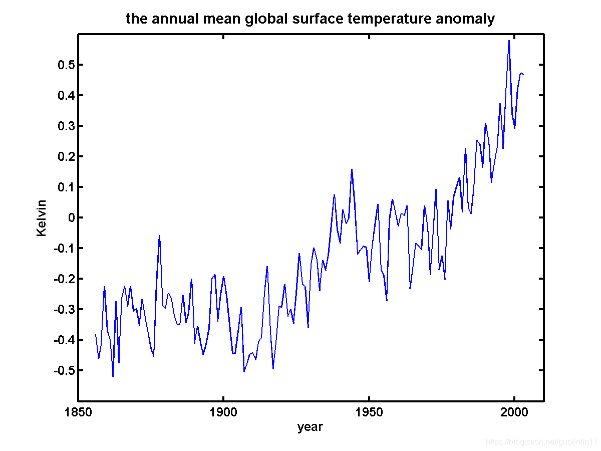
A few examples of how to use these programs are given, with a given dataset “gsta.dat”, which is the annual mean global surface temperature anomaly. In “gsta.dat”, the first column is the time; and the second is the corresponding data value.
1) Load and display data
>> load gsta.dat;
>> plot(gsta(:,1),gsta(:,2));
>> axis([1850 2010 -0.6 0.6]);
>> title('the annual mean global surface temperature anomaly')
>> xlabel('year')
>> ylabel('Kelvin')
2) Using the program as a traditional EMD tool
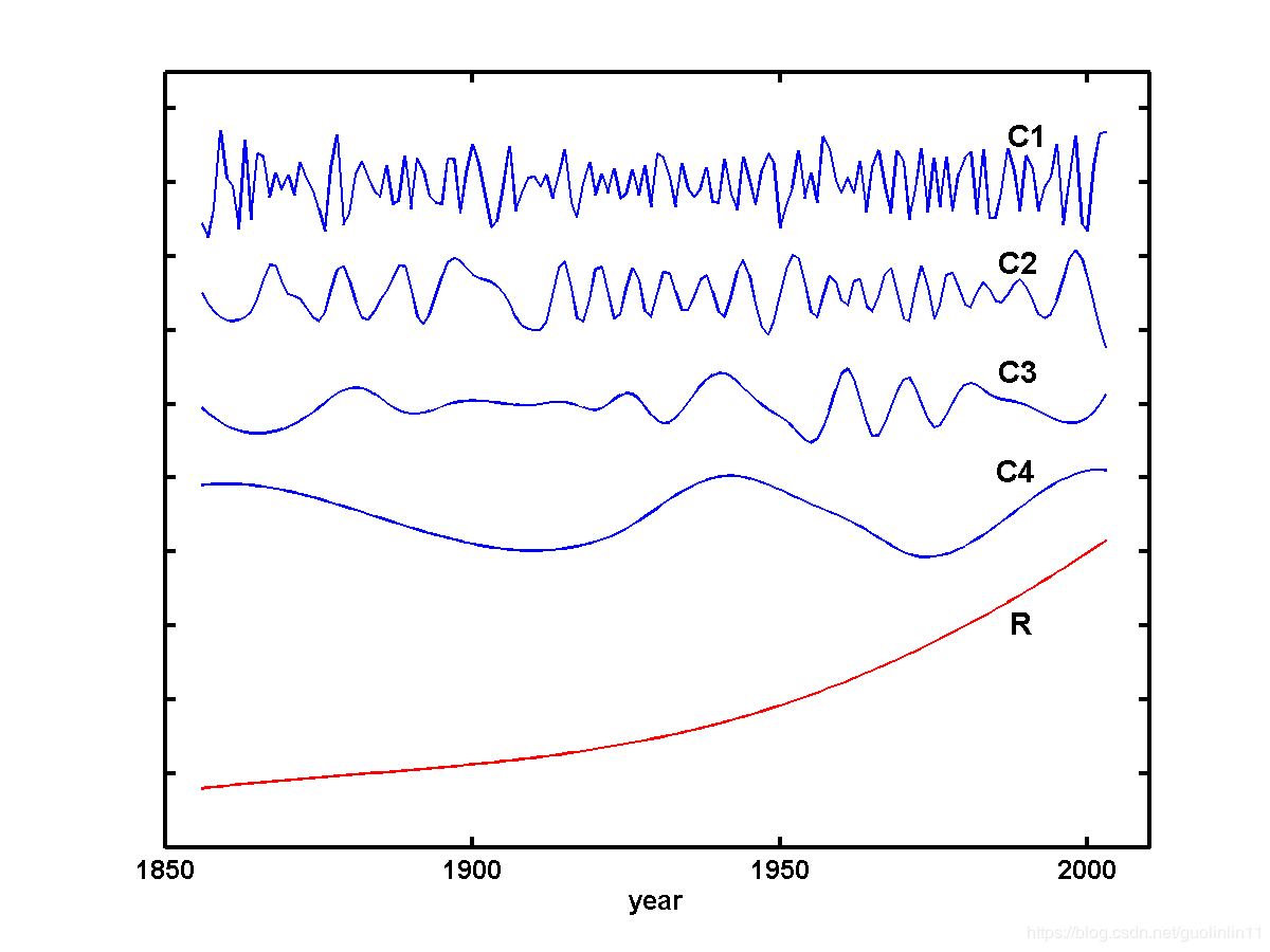
The eemd.m can be used as an EMD decomposition tool:
>> year=gsta(:,1);
>> inData=gsta(:,2);
>> rslt=eemd(inData,0,1);
>> plot(year,rslt(:,2));
>> hold on;
>> plot(year,rslt(:,3)-0.3);
>> plot(year,rslt(:,4)-0.6);
>> plot(year,rslt(:,5)-0.9);
>> plot(year,sum(rslt(:,6:8),2)-1.3,'r-');
>> hold off
>> set(gca,'yTickLabel',[]);
>> axis([1850 2010 -1.8 0.3]);
>> xlabel('year');
“relt” is a matrix containing the decomposition results, with the first column the original input (“gsta(:,2)”) and the last column the trend. In between are the IMFs of frequencies from high to low.
It should be noted that since in the eemd.m, the total number of IMFs m is specified as log2(N)-1, in some occasions (such as the one in this example), the components may be excessively extracted. In these cases, the sum of the latest columns may already satisfy the definition of a trend.
3) Instantaneous frequency of an IMF
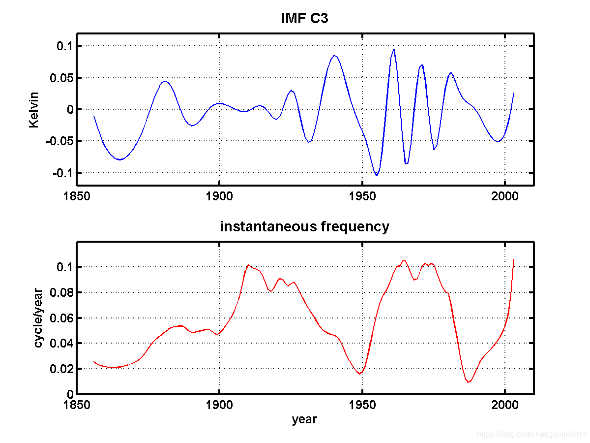
The instantaneous frequency can be obtained through calling ifndq.m function:
>> omega_m3=ifndq(rslt(:,4),1);
>> subplot(2,1,1);
>> plot(year,rslt(:,4));
>> axis([1850 2010 -0.12 0.12]);
>> title('IMF C3');
>> ylabel('Kelvin');
>> grid;
>> subplot(2,1,2);
>> plot(year, omega_m3/2/pi,'r-');
>> grid;
>> xlabel('year');
>> ylabel('cycle/year');
>> title('instantaneous frequency');
>> axis([1850 2010 0 0.12]);
It should be noted that the instantaneous frequency calculation program is not suitable for under sampled oscillations, such as the first IMF (with an averaged period about 3 data points). However, for such under sampled oscillations, the instantaneous frequency is no longer “instantaneous” any way, and any method used to obtain such a quantity will have big errors.
4) Using the program as a EEMD tool
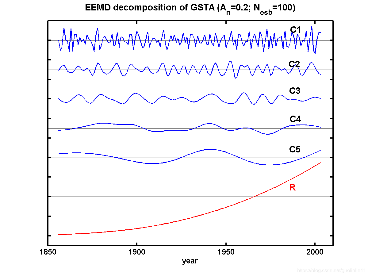
The eemd.m can be used as an EEMD decomposition tool. In this case, the noise assed has an amplitude (standard deviation) of 0.2 of the standard deviation of the linearly detrended annual mean global surface temperature anomaly; and the number of ensemble is 100:
>> rslt=eemd(inData,0.2,100);
>> t(1)=1850;
>> t(2)=2010;
>> y1(1)=0;
>> y1(2)=0;
>> y2(1)=-0.3;
>> y2(2)=-0.3;
>> y3(1)=-0.6;
>> y3(2)=-0.6;
>> y4(1)=-0.9;
>> y4(2)=-0.9;
>> y5(1)=-1.2;
>> y5(2)=-1.2;
>> y6(1)=-1.6;
>> y6(2)=-1.6;
>> plot(t,y1,'k-');
>> hold on;
>> plot(t,y2,'k-');
>> plot(t,y3,'k-');
>> plot(t,y4,'k-');
>> plot(t,y5,'k-');
>> plot(t,y6,'k-');
>> plot(year,rslt(:,1));
>> plot(year,rslt(:,3)-0.3);
>> plot(year,rslt(:,4)-0.6);
>> plot(year,rslt(:,5)-0.9);
>> plot(year,rslt(:,6)-1.2);
>> plot(year,sum(rslt(:,7:8),2)-1.6,'r-');
>> set(gca,'yTickLabel',[]);
>> title('EEMD decomposition of GSTA (A_n=0.2; N_e_s_b=100)')
>> axis([1850 2010 -2.1 0.2]);
>> xlabel('year');
5) Statistical significance test
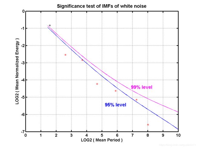
Since the annual mean global surface temperature anomaly behaves completely different from a white noise series, we use computer generated white noise to illustrate how the significance.m can be used:
>> clear;
>> clf;
>> data=randn(512,1);
>> rslt=eemd(data,0,1);
>> imfs=rslt(:,2:8);
>> [sigline95,logep]=significance(imfs,0.05);
>> [sigline99,logep]=significance(imfs,0.01);
>> plot(sigline95(:,1),sigline95(:,2)); % 95 percenta line
>> hold on
>> plot(sigline99(:,1),sigline99(:,2),'m-'); % 99 percenta line
>> plot(logep(:,1),logep(:,2),'r*');
>> plot(logep(1,1),logep(1,2),'k*');
>> grid;
>> xlabel('LOG2 ( Mean Period )');
>> ylabel('LOG2 ( Mean Normalized Energy )');
>> title('Significance test of IMFs of white noise');
>> axis([0 10 -7 0])
3) Trend and detrending
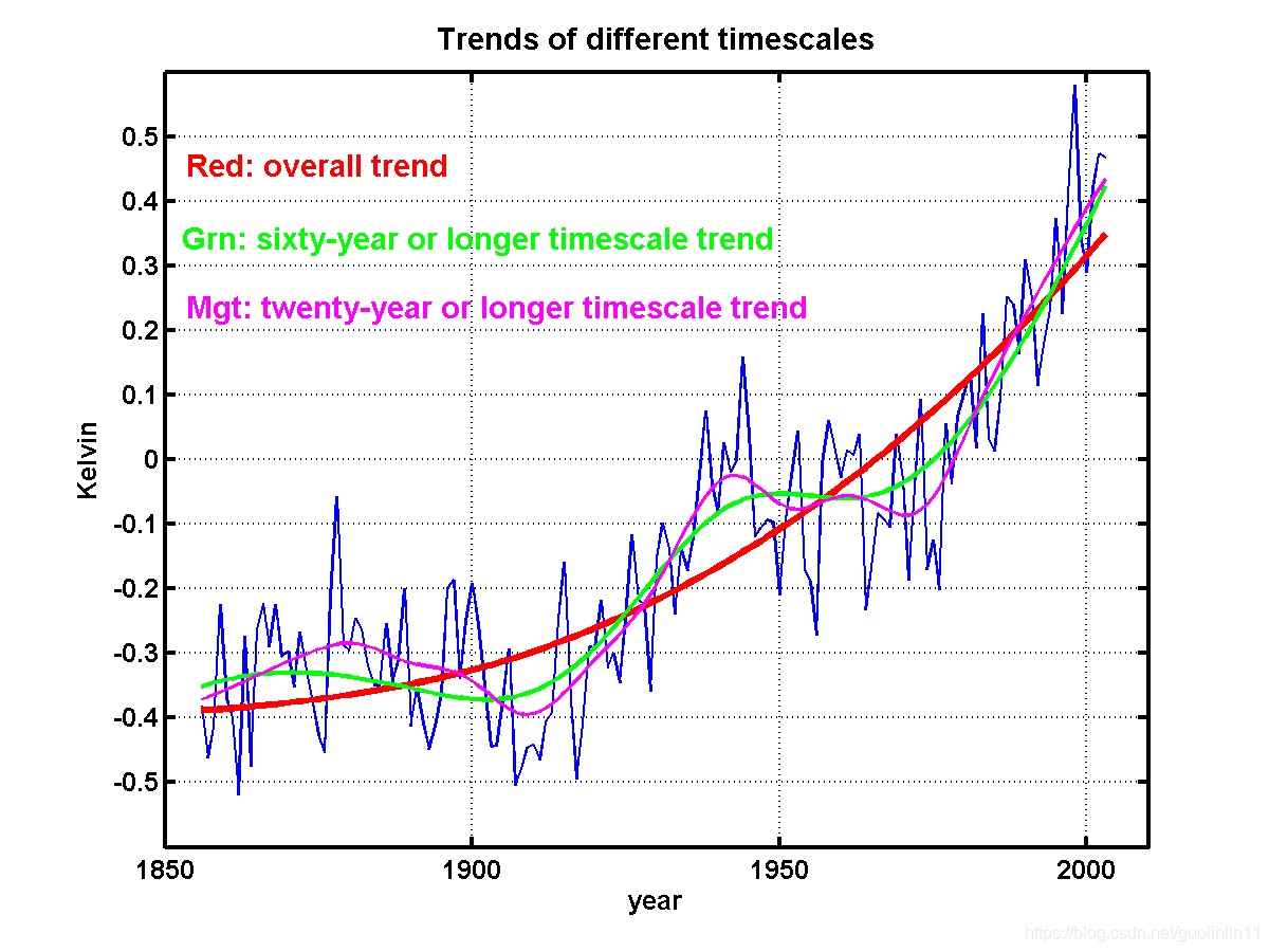
For example, in the previous decomposition, the sum of the last three columns satisfies the definition of trend well.
>> plot(year, rslt(:,1));
>> hold on;
>> plot(year, sum(rslt(:,7:8),2),'r-');
>> plot(year, sum(rslt(:,6:8),2),'g-');
>> plot(year, sum(rslt(:,5:8),2),'m-');
>> title('Trends of different timescales');
>> ylabel('Kelvin');
>> xlabel('year');
>> grid;
参考:
[1]http://rcada.ncu.edu.tw/research1_clip_ex.htm
[2]http://rcada.ncu.edu.tw/research1.htm
