在Frenet坐标系下的动态障碍物避障
本文介绍如何实现基于Frenet坐标系的动态障碍物避障。其中包括:
- cubic spline generation
- Frenet transformation to gloval coordnates
- sampling-based search method
- Bezier curve
- cost function formalization
- lazy collision checking
- pure pursuit trajectory tracking
cubic soline generation
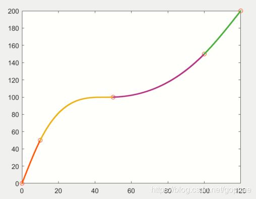
对于给定的一连串waypoints我们需要对其进行平滑线处理,这里介绍一种三阶spline的平滑方法:
function [Px,Py,YAW] = cubic_spline(x,y,MAX_ROAD_WIDTH)
   figure
%     plot(x,y,'ro');
    hold on

    N = length(x);
   A = zeros(N,N);
   B = zeros(N,1);

   for i = 1:N-1
   h(i) = x(i+1) - x(i);
   end

   A(1,1) = 1;
   A(N,N) = 1;
   for i = 2:N-1
       A(i,i) = 2*(h(i-1) + h(i));
   end

   for i  =2 : N-1
   A(i, i+1) = h(i);
   end

   for i  = 2: N-1
       A(i,i-1) = h(i-1);
   end

   for i = 2:N-1
       B(i) = 6* (y(i+1)-y(i))/h(i) - 6* (y(i)-y(i-1))/h(i-1);
   end
   m= A\B

   for i = 1:N
       a(i) = y(i);
   end

     for i = 1:N
       c(i) = m(i)/2;
     end

      for i = 1:N-1
          d(i) =( c(i+1)-c(i) )/(3*h(i));
      end

       for i = 1:N-1
           b(i)  = (a(i+1)-a(i))/h(i)- h(i)/3*(c(i+1)+ 2*c(i));
       end
       Px= [];
       Py = [];
       for  i= 1:N-1
           X = x(i):0.1:x(i+1);
           Y = a(i)+ b(i)*(X-x(i)) + c(i) * (X- x(i)).^2 + d(i) * (X - x(i)).^3;
           Px = [Px,X];
           Py = [Py,Y];
       plot(X, Y,'g-','LineWidth',3)
       plot(X, Y+MAX_ROAD_WIDTH,'r-','LineWidth',2)
       plot(X, Y-MAX_ROAD_WIDTH,'r-','LineWidth',2)
       end

       for i = 1: length(Px)-1
           yaw(i) = atan((Py(i+1)-Py(i))/(Px(i+1)- Px(i)));
       end
       yaw(end+1) = yaw(end);
        YAW =   yaw;
%        s = zeros(length(Px),1);
%        s(1) = 0;
%        for i = 2: length(Px)
%            s(i) = sqrt((Px(i)-Px(i-1)^2+ Py(i)-Py(i-1)^2);
%            s(i) =s(i-1) +
%        end
end
对于一串原始的reference line 参考线点集,我们可以通过三阶曲线拟合将这些点拟合成连续光滑的三阶曲线,这个曲线至少是二阶C1连续的。
Frenet transformation to gloval coordnates
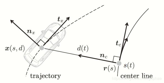
Frenet 坐标系也称道路坐标系,或SL坐标系。之所以使用这样的坐标系,是因为我们在实施规划曲线的时候是以道路为前提的,也就是说,生成的曲线最后都是可以被表达成从当前车辆位置所在的参考线索引位置指向参考线前进方向的新的曲线,而这些新的曲线的参考线前进方向可以用参参考线积分所得的弧线长度表示,也就是S, 而法向,则可以用距离参考线的横向距离来表示也就是L。一旦我们规划的曲线能够在道路坐标系下表示出来,我们就可以通过向量计算获得这个曲线在全局坐标系下的表示。
![]()
可以看到,从Frenet坐标系转向全局坐标系的向量表示由横纵向两部分组成。一个是参考线前进方向,r的方向。另一个就是横向偏移的方向。也就是n法向。
function [waypoint] = frenet_to_global (cx, cy,YAW, location_ind,P) % waypoint generate a 2 by n matrix
waypoint = [];
for i  = 1 : length(location_ind)
    theta = YAW(location_ind(i)) + pi/2;
    waypoint(1, i) = cx(location_ind(i)) + cos(theta) * P(i,2);
    waypoint(2, i) = cy(location_ind(i)) + sin(theta) * P(i,2);
end
% for i = 1: length(location_ind)-1
%     T = [cx(location_ind(i+1))-cx(location_ind(i)) ; cy(location_ind(i+1))-cy(location_ind(i))];
%     theta = atan(cy(location_ind(i+1))-cy(location_ind(i))/cx(location_ind(i+1))-cx(location_ind(i)));
%     R = [cos(theta),-sin(theta); sin(theta), cos(theta)];
%     trans = [R T; 0 0 1];
%     waypoint(:,i) = trans * [P(i,1); P(i,2);1];
%
% end
end
函数frenet_to_global简单的介绍了坐标转化的过程。转化的原理很简单,首先找到frenet坐标系下面的点对应于reference line上面的点,再从这个点向n法向偏移对应的d的距离。theta就是计算出法向的偏移方向。而函数中的location_ind是一个坐标序列号储存矩阵,里面存放着我们规划出的曲线在对应的参考线上最近点的索引号。事实上,我们在规划出连续的贝塞尔曲线后,使用参考线的采样频率对曲线离散化,获得S方向的索引号,以及对应这些点的法向偏移量L。索引位置时,这些信息被存放在P中,P的第二列就是横向偏移量。
    while  s<= Ti
    p(i,:)= Bezierfrenet(D0, Ti, Di,s);
    target_speed =  target_speed;
    location_ind(i) = S;
    s = s + sqrt((cx(S+1)-cx(S))^2 +  (cy(S+1)-cy(S))^2);
    S = S+1;
    i = i+1;
    end
另外一个问题,就是需要对规划出来的曲线进行参考线方向的积分,这个也直接影响到我们在参考线方向积分的距离,这些存储下来的点将被存放在P矩阵中。
sampling-based search method
samling-based search method结构上将位置和车速规划进行了分离。位置上使用了基于贝塞尔曲线的采样撒点,生成曲线,计算cost function, 进行碰撞检测,最后搜索出最优安全曲线。车速上,使用了ACC控制器,在纵向发布一个期望车速计算出期望加速度。
- 贝塞尔曲线
贝塞尔曲线的相关知识可以参考我以前的文章:
Bezier(贝塞尔)曲线的轨迹规划在自动驾驶中的应用(一)
Bezier(贝塞尔)曲线的轨迹规划在自动驾驶中的应用(二)
Bezier(贝塞尔)曲线的轨迹规划在自动驾驶中的应用(三)
Bezier(贝塞尔)曲线(三阶)的轨迹规划在自动驾驶中的应用(四)
Bezier(贝塞尔)曲线(五阶)的轨迹规划在自动驾驶中的应用(五)
Bezier(贝塞尔)曲线(五阶)的轨迹规划在自动驾驶中的应用(六)
贝塞尔曲线的选择,我们进行了对比:
自动驾驶使用贝塞尔曲线进行动态障碍物避障测试
自动驾驶实测:贝塞尔曲线静态障碍物避障
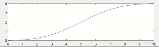
我们通过一个简单的测试函数可以了解贝塞尔曲线:
clc
 clear all


  Ti = 10;
 Di = 4;
 figure
 i = 1;
 for t = 0:0.1: Ti
p(i,:) = Bezierfrenet(Ti, Di,t);

i = i+1;
 end

 figure

plot(p(:,1),p(:,2))
testa = Bezierfrenet(Ti, Di,10)
 function [p] = Bezierfrenet(Ti, Di,t)
 p0 = [ 0, 0];
 p1 = [Ti/2, 0];
 p2= [Ti/2, Di];
 p3 = [Ti, Di];
 %设置控制点

 p= (1-(t)/Ti)^3*p0 + 3*(1-(t)/Ti)^2*(t)/Ti*p1 + 3*(1-(t)/Ti)*((t)/Ti)^2*p2 + ((t)/Ti)^3*p3;

 end
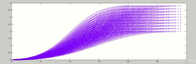
2. 曲线采样(sampling)
我们在Frenet 坐标系下向S方向进行采样。采样方向的距离由短到长采样:
MAXT = 10;% 最大预测 [s]
MINT = 4; % 最小预测 [s]
L方向也是一样,从负最大到正最大:
MAX_ROAD_WIDTH =1.5 ; % 最大道路宽度 [m]
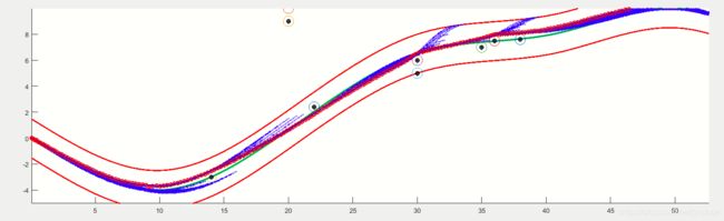
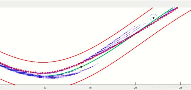
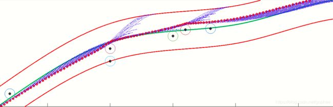
效果如图:
cost function formalization
cost function 选择有很多,具体看我论文:
A Dynamic Motion Planning Framework for Autonomous Driving in Urban Environments
而在本文中,我们只提供简单的cost function fomalization:
% 损失函数权重
KJ = 0.1;
KT = 0.1;
KD = 10;
KLAT = 1.0;
KLON = 1.0;
function [frenet_paths] = calc_frenet_paths(c_d, c_d_d, c_d_dd,MAX_ROAD_WIDTH,...
    D_ROAD_W, MINT,DT,MAXT,KJ,KD,KT)
%    xs = c_d;
%    axs = c_d_dd;
%    axe = 0;
%    vxe = 0;
%    vxs = c_d_d;
% frenet_paths = [];
% tfp = [];
% T = [];
% D = [];
j = 1;
for di = -MAX_ROAD_WIDTH: D_ROAD_W: MAX_ROAD_WIDTH
    for Ti =  MINT: DT: MAXT
           t = 0: DT: Ti; t = t';
%         for i = 1: length(t)
%         p(i,:)= Bezierfrenet(Ti, Di,t(i));
%         end

%         for i = 1: length(t)
%             d_d(i) = calc_first_derivative(a1,a2,a3,a4,a5,t(i));
%         end
%
%         for i = 1: length(t)
%             d_dd(i) = calc_second_derivative(a2,a3,a4,a5,t(i));
%         end
%
%         for i = 1: length(t)
%             d_ddd(i) = calc_third_derivative(a3,a4,a5,t(i));
%         end

%         JP= sum(d_ddd.^2);

        tfp(j) = KT / Ti + KD * abs(di);
        T(j) = Ti;
        D(j) = di;
        j = j+1;
    end
end

frenet_paths = [tfp',T',D'];
frenet_paths = sortrows(frenet_paths);
end
我们在函数中,对曲线进行了离散化,因为cost function需要进行离散化来计算。举个例子,这里我只使用了曲线长度和曲线终点对参考线的偏移量两个指标作为cost function。第一个指标意思是我们更倾向于使用更长的预测距离,这是因为更长的预测距离对远方的障碍物更加敏感,同时稳定性也更高。第二个指标意思是我们倾向于规划出来的轨迹尽量接近于参考线,也就是轨迹尽量是循参考线的迹。代码块中comment掉的一个另一个指标是Jerk,也就是加加速度,用于表征车辆的燃油经济性和驾驶舒适度,这个从曲线角度表示就是对曲线求三阶导数,看三阶导数的连续性。看得出来,计算出三阶导数表达式后,对表达式离散化取值,然后积分获得这一项的cost function.
lazy collision checking
lazy collison checking 是延迟碰撞检测,用于加速碰撞检测,原理上就是碰撞检测独立于cost function, 在计算完cost function后对cost function 进行一次低到高的排序,从头开始进行碰撞检测,一直找到第一个满足碰撞检测的轨迹参数。具体的参考我的论文:A Dynamic Motion Planning Framework for Autonomous Driving in Urban Environments以及自动驾驶中的滞后碰撞检测(lazy-collision-checking)
pure pursuit trajectory tracking
纯跟踪算法,用于解决轨迹跟踪的问题,具体的原理参考Pure Pursuit trajectory tracking and Stanley trajectory tracking总结与比较,相关的测试已经给出:Pure Pursuit纯跟踪算法Python/Matlab算法实现,在本文的测试中,选取了以下部分进行纯跟踪的实现:
function [waypoint] = frenet_to_global (cx, cy,YAW, location_ind,P) % waypoint generate a 2 by n matrix
waypoint = [];
for i  = 1 : length(location_ind)
    theta = YAW(location_ind(i)) + pi/2;
    waypoint(1, i) = cx(location_ind(i)) + cos(theta) * P(i,2);
    waypoint(2, i) = cy(location_ind(i)) + sin(theta) * P(i,2);
end
% for i = 1: length(location_ind)-1
%     T = [cx(location_ind(i+1))-cx(location_ind(i)) ; cy(location_ind(i+1))-cy(location_ind(i))];
%     theta = atan(cy(location_ind(i+1))-cy(location_ind(i))/cx(location_ind(i+1))-cx(location_ind(i)));
%     R = [cos(theta),-sin(theta); sin(theta), cos(theta)];
%     trans = [R T; 0 0 1];
%     waypoint(:,i) = trans * [P(i,1); P(i,2);1];
%
% end
end
function [x, y, yaw, v] = update(x, y, yaw, v, a, delta,dt,L)
    x = x + v * cos(yaw) * dt;
    y = y + v * sin(yaw) * dt;
    yaw = yaw + v / L * tan(delta) * dt;
   v = v + a * dt;
end
function [a] = PIDcontrol(target_v, current_v, Kp,MAX_ACCEL)
a = Kp * (target_v - current_v);
a = min(max(a, -10), MAX_ACCEL);
end
function [ trans] =  BackTransfer(x,y,heading_current)

theta =  heading_current;
R = [cos(theta),-sin(theta); sin(theta), cos(theta)];
xt = x;
yt = y;
T = [xt; yt ] ;
trans = [[R,T];[0,0,1]];
end
function [delta] = pure_pursuit_control(x,y,yaw,v,path_x,path_y,k,Lfc,L,predict)
if predict >length(path_x)
    predict = length(path_x);
end

tx =path_x(predict);
    ty =path_y(predict);
    denom = tx-x;
    if denom == 0
        denom = 0.0001
    end
   alpha =atan(ty-y)/((denom))-yaw;

 Lf = k * v + Lfc;
 delta = atan(2*L * sin(alpha)/Lf)  ;
end
function [lat,current_ind]= calc_current_index(x,y, cx,cy)
N =  length(cx);
Distance = zeros(N,1);
for i = 1:N
Distance(i) =  sqrt((cx(i)-x)^2 + (cy(i)-y)^2);
end
[value, location]= min(Distance);
current_ind = location;
lat = value;
 if cy(current_ind)>y
        lat = - lat;
    else
        lat = lat;
    end
end
function [angle] = pipi(angle)

if (angle > pi)
    angle =  angle - 2*pi;
elseif (angle < -pi)
    angle = angle + 2*pi;
else
    angle = angle;
end
end
最后通过主函数即可调用这些函数对车辆的状态进行实时更新,同时根据实时更新的车辆状态来规划实时路径。
主函数伪代码入下:
while not reach end
	calc_frenet_paths
	calculate lateral_offset, current_ind
	optimal_trajectory = collision_checking_test(candidate_trajectory(frenet_paths))
	calculate acceleration % steering wheel angle
	update vehicle states
end while
最后效果: