【Deep Learning】Variational autoencoder

Original: link

学习变分自编码器（variational autocoder）再一次让我领略到了Bayesian理论的强大之处，variational autocoder是一种powerful的生成模型。

Limitations of autoencoders for content generation

在上期推送的经典的autoencoder中，存在一些局限性，如下

When thinking about it for a minute, this lack of structure among the encoded data into the latent space is pretty normal. Indeed, nothing in the task the autoencoder is trained for enforce to get such organisation: the autoencoder is solely trained to encode and decode with as few loss as possible, no matter how the latent space is organised. Thus, if we are not careful about the definition of the architecture, it is natural that, during the training, the network takes advantage of any overfitting possibilities to achieve its task as well as it can… unless we explicitly regularise it!

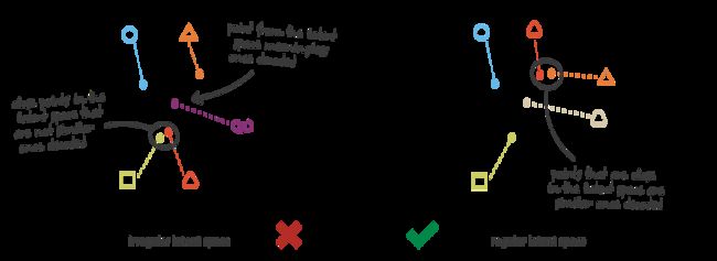
那么，什么式regular和iregular的隐空间呢？

通俗地理解就是在隐空间中输入一个分布中的隐向量进入decoder，decoder能够输出有意义的content，即需要保证隐空间的continuity和completeness，

Definition of variational autoencoder

为了能够充分利用自动编码器的生成目的的解码器，须确保隐空间是足够规则的。一个方法是在训练过程中引入明确的正则化。因此，variational autoencoder可以定义为：

A variational autoencoder can be defined as being an autoencoder whose training is regularised to avoid overfitting and ensure that the latent space has good properties that enable generative process.

Basic architechture of variational autoencoder

Unlike classical (sparse, denoising, etc.) autoencoders, Variational autoencoders (VAEs) are generative models, like Generative Adversarial Networks

首先需要明确的是variational autocoder是一种典型的生成模型，而传统的autoencoder则不是。

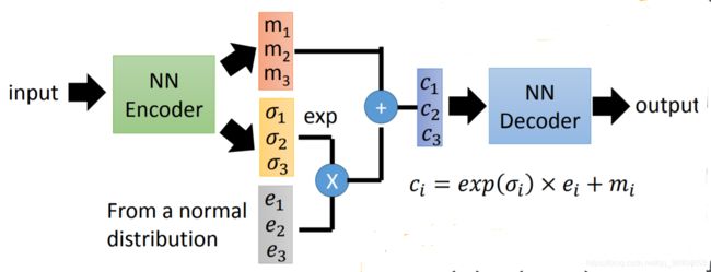
与经典的autoencoder的不同的是，variational autoencoder通过encoder将input编码为隐空间中的一种分布。

Probabilistic framework and assumptions

我们要考虑encoder和decoder的概率模型，即

• Probabilistic encoder: $q(\mathbf{z}|\mathbf{x})$ describes the distribution of the encoded variable given the decoded one.
• Probabilistic decoder: $p(\mathbf{x}|\mathbf{z})$ describes the distribution of the decoded variable given the encoded one.
• Prior distribution: $p(\mathbf{z})$.
• Likelihood: $p(\mathbf{x}|\mathbf{z})$.

下面是关于概率模型的一些假设

• $p(\mathbf{z})$ is a standard Gaussian distribution, i.e.,

$$p(\mathbf{z})\equiv \mathcal{N}(0,\mathbf{I})$$

• $p(\mathbf{x}|\mathbf{z})$ is a Gaussian distribution whose mean is defined by a deterministic function $f$ of the variable of $\mathbf{z}$ and whose covariance matrix has the form of a positive constant $c$ that multiplies the identity matrix $\mathbf{I}$.

$$p(\mathbf{x}|\mathbf{z})\equiv \mathcal{N}(f(\mathbf{z}),c\mathbf{I})$$

Variational inference

In statistics, variational inference (VI) is a technique to approximate complex distributions.

$$\begin{gathered} KL(q_{\lambda }(z\mid x)\mid \mid p(z\mid x))={\mathbf{E}}_q[\log q_{\lambda }(z\mid x)]-{\mathbf{E}}_q[\log p(x,z)] \\ +\log p(x)Eq[logq\lambda (z\mid x)]-Eq[logp(x,z)]+logp(x) \end{gathered}$$

Loss
$$\mathcal{L}(\varphi ,\theta ,\mathbf{x})=D_{\mathrm{K}\mathrm{L}}(q_{\varphi }(\mathbf{h}|\mathbf{x})\Vert p_{\theta }(\mathbf{h}))-{\mathbb{E}}_{q_{\varphi }(\mathbf{h}|\mathbf{x})}(\log p_{\theta }(\mathbf{x}|\mathbf{h}))$$
Here, $D_{KL}$ stands for the Kullback–Leibler divergence.

In mathematical statistics, the Kullback–Leibler divergence is a measure of how one probability distribution is different from a second, reference probability distribution.

Example on Minist

参考例程如下：

'''
  Variational Autoencoder (VAE) with the Keras Functional API.
'''

import keras
from keras.layers import Conv2D, Conv2DTranspose, Input, Flatten, Dense, Lambda, Reshape
from keras.layers import BatchNormalization
from keras.models import Model
from keras.datasets import mnist
from keras.losses import binary_crossentropy
from keras import backend as K
import numpy as np
import matplotlib.pyplot as plt

plt.rc('text', usetex=True)
plt.rc('font', family='serif')
plt.rc('font', size = 16)

# Load MNIST dataset
(input_train, target_train), (input_test, target_test) = mnist.load_data()

# Data & model configuration
img_width, img_height = input_train.shape[1], input_train.shape[2]
batch_size = 128
no_epochs = 100
validation_split = 0.2
verbosity = 1
latent_dim = 2
num_channels = 1

# Reshape data
input_train = input_train.reshape(input_train.shape[0], img_height, img_width, num_channels)
input_test = input_test.reshape(input_test.shape[0], img_height, img_width, num_channels)
input_shape = (img_height, img_width, num_channels)

# Parse numbers as floats
input_train = input_train.astype('float32')
input_test = input_test.astype('float32')

# Normalize data
input_train = input_train / 255
input_test = input_test / 255

# # =================
# # Encoder
# # =================

# Definition
i       = Input(shape=input_shape, name='encoder_input')
cx      = Conv2D(filters=8, kernel_size=3, strides=2, padding='same', activation='relu')(i)
cx      = BatchNormalization()(cx)
cx      = Conv2D(filters=16, kernel_size=3, strides=2, padding='same', activation='relu')(cx)
cx      = BatchNormalization()(cx)
x       = Flatten()(cx)
x       = Dense(20, activation='relu')(x)
x       = BatchNormalization()(x)
mu      = Dense(latent_dim, name='latent_mu')(x)
sigma   = Dense(latent_dim, name='latent_sigma')(x)

# Get Conv2D shape for Conv2DTranspose operation in decoder
conv_shape = K.int_shape(cx)

# Define sampling with reparameterization trick
def sample_z(args):
  mu, sigma = args
  batch     = K.shape(mu)[0]
  dim       = K.int_shape(mu)[1]
  eps       = K.random_normal(shape=(batch, dim))
  return mu + K.exp(sigma / 2) * eps

# Use reparameterization trick to ....??
z       = Lambda(sample_z, output_shape=(latent_dim, ), name='z')([mu, sigma])

# Instantiate encoder
encoder = Model(i, [mu, sigma, z], name='encoder')
encoder.summary()

# =================
# Decoder
# =================

# Definition
d_i   = Input(shape=(latent_dim, ), name='decoder_input')
x     = Dense(conv_shape[1] * conv_shape[2] * conv_shape[3], activation='relu')(d_i)
x     = BatchNormalization()(x)
x     = Reshape((conv_shape[1], conv_shape[2], conv_shape[3]))(x)
cx    = Conv2DTranspose(filters=16, kernel_size=3, strides=2, padding='same', activation='relu')(x)
cx    = BatchNormalization()(cx)
cx    = Conv2DTranspose(filters=8, kernel_size=3, strides=2, padding='same',  activation='relu')(cx)
cx    = BatchNormalization()(cx)
o     = Conv2DTranspose(filters=num_channels, kernel_size=3, activation='sigmoid', padding='same', name='decoder_output')(cx)

# Instantiate decoder
decoder = Model(d_i, o, name='decoder')
decoder.summary()

# =================
# VAE as a whole
# =================

# Instantiate VAE
vae_outputs = decoder(encoder(i)[2])
vae         = Model(i, vae_outputs, name='vae')
vae.summary()

# Define loss
def kl_reconstruction_loss(true, pred):
  # Reconstruction loss
  reconstruction_loss = binary_crossentropy(K.flatten(true), K.flatten(pred)) * img_width * img_height
  # KL divergence loss
  kl_loss = 1 + sigma - K.square(mu) - K.exp(sigma)
  kl_loss = K.sum(kl_loss, axis=-1)
  kl_loss *= -0.5
  # Total loss = 50% rec + 50% KL divergence loss
  return K.mean(reconstruction_loss + kl_loss)

# Compile VAE
vae.compile(optimizer='adam', loss=kl_reconstruction_loss)

# Train autoencoder
vae.fit(input_train, input_train, epochs = no_epochs, batch_size = batch_size, validation_split = validation_split)

# =================
# Results visualization
# Credits for original visualization code: https://keras.io/examples/variational_autoencoder_deconv/
# (François Chollet).
# Adapted to accomodate this VAE.
# =================
def viz_latent_space(encoder, data):
  input_data, target_data = data
  mu, _, _ = encoder.predict(input_data)
  plt.figure(figsize=(8, 10))
  plt.scatter(mu[:, 0], mu[:, 1], c=target_data)
  plt.xlabel('z - dim 1')
  plt.ylabel('z - dim 2')
  plt.colorbar()
  plt.show()

def viz_decoded(encoder, decoder, data):
  num_samples = 15
  figure = np.zeros((img_width * num_samples, img_height * num_samples, num_channels))
  grid_x = np.linspace(-4, 4, num_samples)
  grid_y = np.linspace(-4, 4, num_samples)[::-1]
  for i, yi in enumerate(grid_y):
      for j, xi in enumerate(grid_x):
          z_sample = np.array([[xi, yi]])
          x_decoded = decoder.predict(z_sample)
          digit = x_decoded[0].reshape(img_width, img_height, num_channels)
          figure[i * img_width: (i + 1) * img_width,
                  j * img_height: (j + 1) * img_height] = digit
  plt.figure(figsize=(10, 10))
  start_range = img_width // 2
  end_range = num_samples * img_width + start_range + 1
  pixel_range = np.arange(start_range, end_range, img_width)
  sample_range_x = np.round(grid_x, 1)
  sample_range_y = np.round(grid_y, 1)
  plt.xticks(pixel_range, sample_range_x)
  plt.yticks(pixel_range, sample_range_y)
  plt.xlabel('z - dim 1')
  plt.ylabel('z - dim 2')
  # matplotlib.pyplot.imshow() needs a 2D array, or a 3D array with the third dimension being of shape 3 or 4!
  # So reshape if necessary
  fig_shape = np.shape(figure)
  if fig_shape[2] == 1:
    figure = figure.reshape((fig_shape[0], fig_shape[1]))
  # Show image
  plt.imshow(figure)
  plt.show()

# Plot results
data = (input_test, target_test)
viz_latent_space(encoder, data)
viz_decoded(encoder, decoder, data)

下为运行100代得到的结果

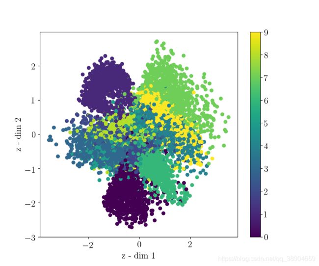
• We will visualize our test set inputs mapped onto the latent space. This allows us to check the continuity and completeness of our latent space.
  

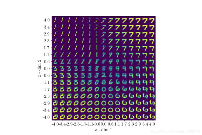
• We will also visualize an uniform walk across latent space to see how sampling from it will result in output that actually makes sense. This is actually the end result we’d love to see

Discriminative model & generative model

关于discriminative model和generative model的区别，请看下句

Differently from discriminative modeling that aims to learn a predictor given the observation, generative modeling tries to simulate how the data is generated, in order to understand the underlying causal relations. ref

更具体的区别见下表

通俗地讲，判别模型旨在学习一个boundary进行分类，生成模型旨在建模每个类别样本的分布，