The Haar Transform 哈尔变化

Probably the simplest useful energy compression process is the Haar transform. In 1-dimension, this transforms a 2-element vector  (x(1)x(2))T  into  (y(1)y(2))T using:

(y(1)y(2))=T(x(1)x(2))

(1)

where  T=12√(111-1) . Thus  y(1)  and  y(2)  are simply the sum and difference of  x(1)  and  x(2) , scaled by  12√  to preserve energy.

Note that  T  is an orthonormal matrix because its rows are orthogonal to each other (their dot products are zero) and they are normalised to unit magnitude. Therefore T-1=TT . (In this case  T  is symmetric so  TT=T .) Hence we may recover  x  from  y  using:

(x(1)x(2))=TT(y(1)y(2))

(2)

In 2-dimensions  x  and  y  become  2×2  matrices. We may transform first the columns of  x , by premultiplying by  T , and then the rows of the result by postmultiplying by  TT . Hence:

y=TxTT

(3)

and to invert:

x=TTyT

(4)

To show more clearly what is happening:

If

x=(acbd)

then

y=12(a+b+c+da+b−c−da−b+c−da−b−c+d)

These operations correspond to the following filtering processes:

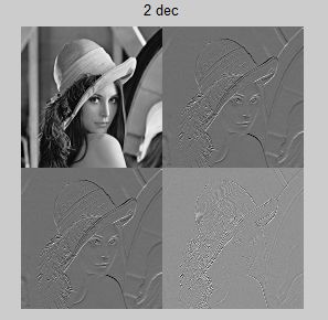
• Top left:  a+b+c+d  = 4-point average or 2-D lowpass (Lo-Lo) filter.
• Top right:  a−b+c−d  = Average horizontal gradient or horizontal highpass and vertical lowpass (Hi-Lo) filter.
• Lower left:  a+b−c−d  = Average vertical gradient or horizontal lowpass and vertical highpass (Lo-Hi) filter.
• Lower right:  a−b−c+d  = Diagonal curvature or 2-D highpass (Hi-Hi) filter.

To apply this transform to a complete image, we group the pels into  2×2  blocks and apply  Equation 3 to each block. The result (after reordering) is shown in  Figure 1(B). To view the result sensibly, we have grouped all the top left components of the  2×2  blocks in  y  together to form the top left subimage in  Figure 1(B), and done the same for the components in the other 3 positions to form the corresponding other 3 subimages.

It is clear from  Figure 1(B) that most of the energy is contained in the top left (Lo-Lo) subimage and the least energy is in the lower right (Hi-Hi) subimage. Note how the top right (Hi-Lo) subimage contains the near-vertical edges and the lower left (Lo-Hi) subimage contains the near-horizontal edges.

The energies of the subimages and their percentages of the total are:

TABLE 1

Lo-Lo	Hi-Lo	Lo-Hi	Hi-Hi
201.73×106	4.56×106	1.89×106	0.82×106
96.5%	2.2%	0.9%	0.4%

Total energy in Figure 1(A) and Figure 1(B) =  208.99×106 .

We see that a significant compression of energy into the Lo-Lo subimage has been achieved. However the energy measurements do not tell us directly how much data compression this gives.

A much more useful measure than energy is the entropy of the subimages after a given amount of quantisation. This gives the minimum number of bits per pel needed to represent the quantised data for each subimage, to a given accuracy, assuming that we use an ideal entropy code. By comparing the total entropy of the 4 subimages with that of the original image, we can estimate the compression that one level of the Haar transform can provide.

http://cnx.org/content/m11087/latest/  英文原文地址

function [f1,f2,f3,f4]=myhaar_2d(f,n)
        % n=1,2,3,4 n次分解   
        % f 为 输入的图片矩阵
        % f1 近似 f2 水平细节 f3 垂直细节 f4 对角细节
        P=size(f);
        G=[];
        k=2^n;   
        T1 = haar_kron(k);  % 计算haar 矩阵
        if mod(P(1),k)|| mod(P(2),k)    %  如果矩阵维度不为k 的倍数，则填充零到k 的倍数
           G1=zeros((fix(P(1)/k)+1)*k,(fix(P(2)/k)+1)*k);
           G1(1:P(1),1:P(2))=f;
        else     % 如果矩阵维度为k 的倍数
            G1=f; 
        end
        for i=1:size(G1,1)/k
            for j=1:size(G1,2)/k
            x1=(i-1)*k;
            x2=(j-1)*k;
            TT=T1*G1(x1+1:x1+k,x2+1:x2+k)*T1'; % 把图像分成很多小子块，对每一块 A 进行haar 矩阵变换  Y=T*A*T'
            % haar 反变换 为 A=T'*Y*T
            G(x1+1:x1+k,x2+1:x2+k)=TT;
            end
        end
        f1=G(1:k:end,1:k:end);  %取近似 
        f3=G(1:k:end,2:k:end);  %取水平系数
        f2=G(2:k:end,1:k:end);  %取垂直系数
        f4=G(2:k:end,2:k:end);  %取对角系数
        f1=mat2gray(f1);      % 矩阵归一化
        f2=mat2gray(f2);
        f3=mat2gray(f3);
        f4=mat2gray(f4);
end

function y=haar_kron(N)
%  2^n=N ,n=1,2,3·······
y=1;
a=[1,1];
b=[1,-1];
k=1;
while(k

 I=im2double(imread('lenna.tif'));
 figure,imshow(I);title('original img');
 for i=1:2
    [f1,f2,f3,f4]=myhaar_2d(I,i);
    ff=[f1,f2;f3,f4];
    figure,imshow(ff);
 end
 % matlab 中已有的二维小波多级分解函数
wname='db1';  
[c,s]=wavedec2(I,2,wname);  % 二级 db1 小波(haar wavelet)分解


ca1=appcoef2(c,s,wname,1); % 一级近似
ch1=detcoef2('h',c,s,1);   % 一级水平细节
cv1=detcoef2('v',c,s,1);   % 一级垂直细节
cd1=detcoef2('d',c,s,1);   % 一级对角细节

ca1=mat2gray(ca1);     % 归一化
ch1=mat2gray(ch1);
cv1=mat2gray(cv1);
cd1=mat2gray(cd1);
figure,imshow([ca1,ch1;cv1,cd1]);title(' 1 dec'); % 一级分解

ca2=appcoef2(c,s,wname,2);   % 二级
ch2=detcoef2('h',c,s,2);
cv2=detcoef2('h',c,s,2);
cd2=detcoef2('d',c,s,2);
ca2=mat2gray(ca2);
ch2=mat2gray(ch2);
cv2=mat2gray(cv2);
cd2=mat2gray(cd2);
figure,imshow([ca2,ch2;cv2,cd2]); title('2 dec');

参考资料：http://fourier.eng.hmc.edu/e161/lectures/Haar/index.html

               http://en.wikipedia.org/wiki/Haar_wavelet

               http://cm.bell-labs.com/who/wim/papers/athome/haar.pdf

有用的一些网站

http://www.multires.caltech.edu/teaching/courses/waveletcourse/

http://cm.bell-labs.com/who/wim/papers/athome/