在Fashion_MNIST数据集上使用Convolutions（卷积层）来优化计算机视觉

使用卷积来提高计算机视觉精度

一、在原来的DNN(深度神经网络)上加上卷积层，构成深度卷积神经网络。

1、原DNN深度神经网络模型

import tensorflow as tf
mnist = tf.keras.datasets.fashion_mnist
(training_images,training_labels),(test_images,test_labels) =mnist.load_data()
training_images = training_images / 255.0
test_images = test_images / 255.0
model = tf.keras.models.Sequential([
    tf.keras.layers.Flatten(),
    tf.keras.layers.Dense(128, activation=tf.nn.relu),
    tf.keras.layers.Dense(10, activation=tf.nn.softmax)
])
model.compile(optimizer='adam', loss='sparse_categorical_crossentropy',metrics=['accuracy'])
model.fit(training_images, training_labels, epochs=5)

test_loss = model.evaluate(test_images,test_labels)

WARNING:tensorflow:From E:\anaconda3\Anaconda\lib\site-packages\tensorflow\python\ops\resource_variable_ops.py:435: colocate_with (from tensorflow.python.framework.ops) is deprecated and will be removed in a future version.
Instructions for updating:
Colocations handled automatically by placer.
Epoch 1/5
60000/60000 [==============================] - 5s 80us/sample - loss: 0.4973 - acc: 0.8264
Epoch 2/5
60000/60000 [==============================] - 5s 79us/sample - loss: 0.3707 - acc: 0.8679
Epoch 3/5
60000/60000 [==============================] - 4s 75us/sample - loss: 0.3331 - acc: 0.8791
Epoch 4/5
60000/60000 [==============================] - 5s 81us/sample - loss: 0.3081 - acc: 0.8859
Epoch 5/5
60000/60000 [==============================] - 4s 75us/sample - loss: 0.2941 - acc: 0.8914
10000/10000 [==============================] - 0s 41us/sample - loss: 0.3509 - acc: 0.8768

当加上卷积层Convolutions后的模型，测试其精度

import tensorflow as tf
mnist = tf.keras.datasets.fashion_mnist
(training_images,training_labels),(test_images,test_labels) =mnist.load_data()
### .reshape()转化为4D张量
training_images = training_images.reshape(60000, 28, 28, 1)
training_images = training_images / 255.0
### .reshape()
test_images = test_images.reshape(10000, 28, 28, 1)
test_images = test_images / 255.0
model = tf.keras.models.Sequential([
    ### 加入卷积层
    tf.keras.layers.Conv2D(64, (3, 3), activation='relu', input_shape=(28,28,1)),
    tf.keras.layers.MaxPooling2D(2,2),
    tf.keras.layers.Conv2D(64,(3,3),activation='relu'),
    tf.keras.layers.MaxPooling2D(2,2),
    tf.keras.layers.Flatten(),
    tf.keras.layers.Dense(128, activation=tf.nn.relu),
    tf.keras.layers.Dense(10, activation=tf.nn.softmax)
])
model.compile(optimizer='adam', loss='sparse_categorical_crossentropy',metrics=['accuracy'])
### 使用model.summary()查看每一层输出的模型
model.summary()
model.fit(training_images, training_labels, epochs=5)

test_loss = model.evaluate(test_images,test_labels)

_________________________________________________________________
Layer (type)                 Output Shape              Param #   
=================================================================
conv2d (Conv2D)              (None, 26, 26, 64)        640       
_________________________________________________________________
max_pooling2d (MaxPooling2D) (None, 13, 13, 64)        0         
_________________________________________________________________
conv2d_1 (Conv2D)            (None, 11, 11, 64)        36928     
_________________________________________________________________
max_pooling2d_1 (MaxPooling2 (None, 5, 5, 64)          0         
_________________________________________________________________
flatten_1 (Flatten)          (None, 1600)              0         
_________________________________________________________________
dense_2 (Dense)              (None, 128)               204928    
_________________________________________________________________
dense_3 (Dense)              (None, 10)                1290      
=================================================================
Total params: 243,786
Trainable params: 243,786
Non-trainable params: 0
_________________________________________________________________
Epoch 1/5
60000/60000 [==============================] - 68s 1ms/sample - loss: 0.4377 - acc: 0.8402
Epoch 2/5
60000/60000 [==============================] - 69s 1ms/sample - loss: 0.2944 - acc: 0.8915
Epoch 3/5
60000/60000 [==============================] - 68s 1ms/sample - loss: 0.2485 - acc: 0.9078
Epoch 4/5
60000/60000 [==============================] - 68s 1ms/sample - loss: 0.2163 - acc: 0.9190
Epoch 5/5
60000/60000 [==============================] - 69s 1ms/sample - loss: 0.1902 - acc: 0.9288
10000/10000 [==============================] - 4s 418us/sample - loss: 0.2425 - acc: 0.9099

###由上面两个模型的对比可知，CNN网络的准确率得到明显提升，CNN网络提取并加强了图像的特征，说明我们的学习有了正反馈，但是如果当我们继续训练多次，例如20次左右，会发现它的准确性降低了。这样的情况叫做过拟合。
Step 1：You’ll notice that there’s a bit of a change here in that the training data needed to be reshaped. That’s because the first convolution expects a single tensor containing everything, so instead of 60,000 28x28x1 items in a list, we have a single 4D list that is 60,000x28x28x1, and the same for the test images. If you don’t do this, you’ll get an error when training as the Convolutions do not recognize the shape.
Step 2 定义模型：1、卷积核的数量是随机的，但是最好是32的倍数；2、卷积核的大小；3、使用relu激活函数；4、在第一层，输入数据的形状
Step 3：使用MaxPooling层进行卷积，这一层的目的主要是用来压缩图片，以及突显特征
Step 4：增加另一层卷积层
Step 5：使用Flatten()把输出压平，在这以后就拥有了与非卷积版本的DNN相同的结构了
Step 6：编译，调用fit函数进行训练，评估测试集的损失和拟合度

print(test_labels[:100])

[9 2 1 1 6 1 4 6 5 7 4 5 7 3 4 1 2 4 8 0 2 5 7 9 1 4 6 0 9 3 8 8 3 3 8 0 7
 5 7 9 6 1 3 7 6 7 2 1 2 2 4 4 5 8 2 2 8 4 8 0 7 7 8 5 1 1 2 3 9 8 7 0 2 6
 2 3 1 2 8 4 1 8 5 9 5 0 3 2 0 6 5 3 6 7 1 8 0 1 4 2]

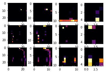
可视化卷积层和池化层

这段代码将以图形方式显示卷积。print (test_labels[;100])显示了测试集中的前100个标签，您可以看到索引0、索引23和索引28处的标签都是相同的值(9)。让我们来看看对它们进行卷积运算的结果，你会开始看到它们之间的共同特征。现在，当DNN对这些数据进行训练时，它处理的数据要少得多，而且它可能会根据这个卷积/池的组合找到鞋子之间的共性。

import matplotlib.pyplot as plt
f, axarr = plt.subplots(3,4)
FIRST_IMAGE=0
SECOND_IMAGE=7
THIRD_IMAGE=26
CONVOLUTION_NUMBER = 1
from tensorflow.keras import models
layer_outputs = [layer.output for layer in model.layers]
activation_model = tf.keras.models.Model(inputs = model.input, outputs = layer_outputs)
for x in range(0,4):
  f1 = activation_model.predict(test_images[FIRST_IMAGE].reshape(1, 28, 28, 1))[x]
  axarr[0,x].imshow(f1[0, : , :, CONVOLUTION_NUMBER], cmap='inferno')
  axarr[0,x].grid(False)
  f2 = activation_model.predict(test_images[SECOND_IMAGE].reshape(1, 28, 28, 1))[x]
  axarr[1,x].imshow(f2[0, : , :, CONVOLUTION_NUMBER], cmap='inferno')
  axarr[1,x].grid(False)
  f3 = activation_model.predict(test_images[THIRD_IMAGE].reshape(1, 28, 28, 1))[x]
  axarr[2,x].imshow(f3[0, : , :, CONVOLUTION_NUMBER], cmap='inferno')
  axarr[2,x].grid(False)

Exercise

1、更换卷积层数，换成16，64，32，看看对时间和准确性有什么影响
2、移除最后一层卷积
3、增加更多的卷积层
4、去掉所有的卷积层，只留下第一层卷积
5、使用callBack函数来检查损失函数，看能否完成任务