cs231n assignment1_Q4_two_layer_net

A two-layer fully-connected neural network. The net has an input dimension of
N, a hidden layer dimension of H, and performs classification over C classes.
We train the network with a softmax loss function and L2 regularization on the
weight matrices. The network uses a ReLU nonlinearity after the first fully
connected layer.In other words, the network has the following architecture:
input - fully connected layer - ReLU - fully connected layer - softmax
The outputs of the second fully-connected layer are the scores for each class.

本次两层网络的作业难点还是在梯度的计算上，题目要求的两个激活函数分别是ReLu函数和softmax函数。来回顾一下。

对其求导

ReLu

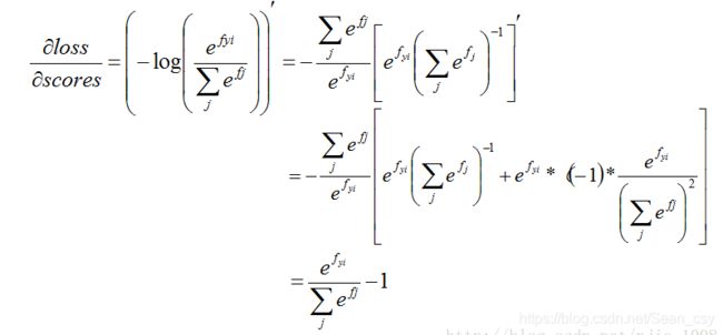
softmax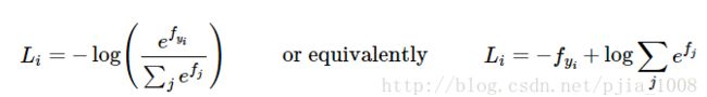

其中，

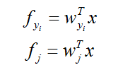
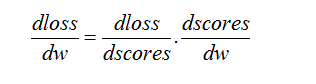
运用链式法则,

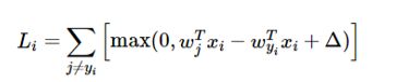
这里求导要进行分类，当j!=yi 时：

当j==yi时：

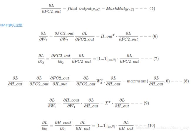
在网络中，我们用反向传播算法来求梯度。以下公式来源（https://blog.csdn.net/yc461515457/article/details/51944683）

前向传播：

反向传播

在明确方法后，开始编写程序。

from __future__ import print_function

import numpy as np
import matplotlib.pyplot as plt
from past.builtins import xrange

class TwoLayerNet(object):
  """
  A two-layer fully-connected neural network. The net has an input dimension of
  N, a hidden layer dimension of H, and performs classification over C classes.
  We train the network with a softmax loss function and L2 regularization on the
  weight matrices. The network uses a ReLU nonlinearity after the first fully
  connected layer.

  In other words, the network has the following architecture:

  input - fully connected layer - ReLU - fully connected layer - softmax

  The outputs of the second fully-connected layer are the scores for each class.
  """

  def __init__(self, input_size, hidden_size, output_size, std=1e-4):
    """
    Initialize the model. Weights are initialized to small random values and
    biases are initialized to zero. Weights and biases are stored in the
    variable self.params, which is a dictionary with the following keys:

    W1: First layer weights; has shape (D, H)
    b1: First layer biases; has shape (H,)
    W2: Second layer weights; has shape (H, C)
    b2: Second layer biases; has shape (C,)

    Inputs:
    - input_size: The dimension D of the input data.
    - hidden_size: The number of neurons H in the hidden layer.
    - output_size: The number of classes C.
    """
    self.params = {}
    self.params['W1'] = std * np.random.randn(input_size, hidden_size)
    self.params['b1'] = np.zeros(hidden_size)
    self.params['W2'] = std * np.random.randn(hidden_size, output_size)
    self.params['b2'] = np.zeros(output_size)

  def loss(self, X, y=None, reg=0.0):
    """
    输入层（D），全连接层-ReLu(H)，softmax(C)
    Compute the loss and gradients for a two layer fully connected neural
    network.

    Inputs:
    - X: Input data of shape (N, D). Each X[i] is a training sample.
    - y: Vector of training labels. y[i] is the label for X[i], and each y[i] is
      an integer in the range 0 <= y[i] < C. This parameter is optional; if it
      is not passed then we only return scores, and if it is passed then we
      instead return the loss and gradients.
    - reg: Regularization strength.

    Returns:
    If y is None, return a matrix scores of shape (N, C) where scores[i, c] is
    the score for class c on input X[i].

    If y is not None, instead return a tuple of:
    - loss: Loss (data loss and regularization loss) for this batch of training
      samples.
    - grads: Dictionary mapping parameter names to gradients of those parameters
      with respect to the loss function; has the same keys as self.params.
    """
    # Unpack variables from the params dictionary
    W1, b1 = self.params['W1'], self.params['b1']
    W2, b2 = self.params['W2'], self.params['b2']
    N, D = X.shape

    # Compute the forward pass
    scores = None
    # fc1_out = X*W1+b1
    # H_out = max(0,fc1_out)
    # fc2_out = H_out*W2+b2
    # final_output = softmax(fc2_out)
    #############################################################################
    # TODO: Perform the forward pass, computing the class scores for the input.
    # 前向传播                                                                   #
    # Store the result in the scores variable, which should be an array of      #
    # shape (N, C).                                                             #
    #############################################################################

    hidden_layer = np.maximum(0, np.dot(X, W1) + b1)  # ReLU activation
    scores = np.dot(hidden_layer, W2) + b2
    print(scores.shape)

    #############################################################################
    #                              END OF YOUR CODE                             #
    #############################################################################
    
    # If the targets are not given then jump out, we're done
    if y is None:
      return scores

    # Compute the loss
    loss = None
    #############################################################################
    # TODO: Finish the forward pass, and compute the loss. This should include  #
    # both the data loss and L2 regularization for W1 and W2. Store the result  #
    # in the variable loss, which should be a scalar. Use the Softmax           #
    # classifier loss.                                                          #
    #############################################################################

    # softmax 损失函数公式
    scores = scores - np.max(scores, axis=1, keepdims=True) #防止指数爆炸
    exp_sum = np.sum(np.exp(scores), axis=1, keepdims=True)
    #loss = -np.sum(scores[range(N), y]) + np.sum(np.log(exp_sum))
    loss = np.sum(-scores[range(N),y] + np.sum(np.log(exp_sum)))
    loss = loss / N + 0.5 * reg * (np.sum(W1 * W1) + np.sum(W2 * W2))

    #############################################################################
    #                              END OF YOUR CODE                             #
    #############################################################################

    # Backward pass: compute gradients
    grads = {} #字典
    #############################################################################
    # TODO: Compute the backward pass, computing the derivatives of the weights #
    # and biases. Store the results in the grads dictionary. For example,       #
    # grads['W1'] should store the gradient on W1, and be a matrix of same size #
    #############################################################################
	
    #计算score梯度 根据softmax求梯度公式。
    #这部分需要重点理解
    prob = np.exp(scores) / exp_sum #求导结果的一项，e^yi/Σe^j
    prob[range(N), y] -= 1  #yi=j时候，求导的结果有个-1项

    dscores= prob / N  #这里注意和softmax里的区分

    #反向传播求梯度
    dW2 = np.dot(hidden_layer.T,dscores)
    db2 = np.sum(dscores, axis=0, keepdims=False)


    dhidden = np.dot(dscores,W2.T)
    dhidden[hidden_layer <= 0] = 0  #max(0, ) 0求导还是0

    dW1 = np.dot(X.T,dhidden)
    db1 = np.sum(dhidden, axis=0, keepdims=False)

    #正则化
    dW2 += reg*W2
    dW1 += reg*W1

    grads['W1'] = dW1
    grads['W2'] = dW2
    grads['b2'] = db2
    grads['b1'] = db1
    #############################################################################
    #                              END OF YOUR CODE                             #
    #############################################################################

    return loss, grads

  def train(self, X, y, X_val, y_val,
            learning_rate=1e-3, learning_rate_decay=0.95,
            reg=5e-6, num_iters=100,
            batch_size=200, verbose=False):
    """
    Train this neural network using stochastic gradient descent.

    Inputs:
    - X: A numpy array of shape (N, D) giving training data.
    - y: A numpy array f shape (N,) giving training labels; y[i] = c means that
      X[i] has label c, where 0 <= c < C.
    - X_val: A numpy array of shape (N_val, D) giving validation data.
    - y_val: A numpy array of shape (N_val,) giving validation labels.
    - learning_rate: Scalar giving learning rate for optimization.
    - learning_rate_decay: Scalar giving factor used to decay the learning rate
      after each epoch.
    - reg: Scalar giving regularization strength.
    - num_iters: Number of steps to take when optimizing.
    - batch_size: Number of training examples to use per step.
    - verbose: boolean; if true print progress during optimization.
    """
    num_train = X.shape[0]
    iterations_per_epoch = max(num_train / batch_size, 1)

    # Use SGD to optimize the parameters in self.model
    loss_history = []
    train_acc_history = []
    val_acc_history = []

    for it in xrange(num_iters):
      X_batch = None
      y_batch = None

      #########################################################################
      # TODO: Create a random minibatch of training data and labels, storing  #
      # them in X_batch and y_batch respectively.                             #
      #########################################################################

      #随机取
      sample_index = np.random.choice(num_train, batch_size, replace=True)
      X_batch = X[sample_index]
      y_batch = y[sample_index]

      #########################################################################
      #                             END OF YOUR CODE                          #
      #########################################################################

      # Compute loss and gradients using the current minibatch
      loss, grads = self.loss(X_batch, y=y_batch, reg=reg)
      loss_history.append(loss)

      #########################################################################
      # TODO: Use the gradients in the grads dictionary to update the         #
      # parameters of the network (stored in the dictionary self.params)      #
      # using stochastic gradient descent. You'll need to use the gradients   #
      # stored in the grads dictionary defined above.                         #
      #########################################################################

      dW1 = grads['W1']
      dW2 = grads['W2']
      db1 = grads['b1']
      db2 = grads['b2']
      self.params['W1'] -= learning_rate * dW1
      self.params['W2'] -= learning_rate * dW2
      self.params['b2'] -= learning_rate * db2
      self.params['b1'] -= learning_rate * db1


      #########################################################################
      #                             END OF YOUR CODE                          #
      #########################################################################

      if verbose and it % 100 == 0:
        print('iteration %d / %d: loss %f' % (it, num_iters, loss))

      # Every epoch, check train and val accuracy and decay learning rate.
      if it % iterations_per_epoch == 0:
        # Check accuracy
        train_acc = (self.predict(X_batch) == y_batch).mean()
        val_acc = (self.predict(X_val) == y_val).mean()
        train_acc_history.append(train_acc)
        val_acc_history.append(val_acc)

        # Decay learning rate
        learning_rate *= learning_rate_decay

    return {
      'loss_history': loss_history,
      'train_acc_history': train_acc_history,
      'val_acc_history': val_acc_history,
    }

  def predict(self, X):
    """
    Use the trained weights of this two-layer network to predict labels for
    data points. For each data point we predict scores for each of the C
    classes, and assign each data point to the class with the highest score.

    Inputs:
    - X: A numpy array of shape (N, D) giving N D-dimensional data points to
      classify.

    Returns:
    - y_pred: A numpy array of shape (N,) giving predicted labels for each of
      the elements of X. For all i, y_pred[i] = c means that X[i] is predicted
      to have class c, where 0 <= c < C.
    """
    y_pred = None

    ###########################################################################
    # TODO: Implement this function; it should be VERY simple!                #
    ###########################################################################

    hidden_lay = np.maximum(0, np.dot(X, self.params['W1']+self.params['b1']))
    y_pred = np.argmax(np.dot(hidden_lay, self.params['W2']), axis=1)
    ###########################################################################
    #                              END OF YOUR CODE                           #
    ###########################################################################

    return y_pred

two_layer_net.ipynb

调优超参数和之前作业类似。

best_net = None # store the best model into this 

#################################################################################
# TODO: Tune hyperparameters using the validation set. Store your best trained  #
# model in best_net.                                                            #
#                                                                               #
# To help debug your network, it may help to use visualizations similar to the  #
# ones we used above; these visualizations will have significant qualitative    #
# differences from the ones we saw above for the poorly tuned network.          #
#                                                                               #
# Tweaking hyperparameters by hand can be fun, but you might find it useful to  #
# write code to sweep through possible combinations of hyperparameters          #
# automatically like we did on the previous exercises.                          #
#################################################################################

best_val = -1
input_size = 32 * 32 * 3
hidden_size = 100
num_classes = 10

net = TwoLayerNet(input_size, hidden_size,num_classes)
learing_rates = [1e-3, 1.5e-3, 2e-3]
regularizations = [0.2, 0.35, 0.5]
for lr in learing_rates:
    for reg in regularizations:
        stats = net.train(X_train, y_train, X_val, y_val,
                          num_iters=1500,batch_size=200,
                          learning_rate=lr,learning_rate_decay=0.95,
                          reg=reg, verbose=False)
        val_acc = (net.predict(X_val) == y_val).mean()
        if val_acc > best_val:
            best_val = val_acc
            best_net = net
        print ("lr ",lr, "reg ", reg, "val accuracy:", val_acc)
print ("best validation accuracyachieved during cross-validation: ", best_val)


#####################################################################。############
#                               END OF YOUR CODE                                #
#################################################################################

最后总结一下，这是我在另外一个博主的文章时觉得不错的话，

Delta = “本地梯度”*“上沿梯度”

有趣的是，变量间做“加法”，传回的梯度都是那份“上沿梯度”，相当于是一个广播器

变量间做“max()”，传回的梯度是那份“上沿梯度”给最大的值，其他的梯度是0，相当于是一个 路由器

变量间做“乘法”，传回的梯度都是那份“上沿梯度”对方本身的值，相当于是一个（带放大“上沿梯度”倍）交换器。

这三个典例，应该能帮助我们直观地理解 backpropagation。