第四章：目标检测YoloV3（中）

单阶段目标检测模型YOLO-V3

上面介绍的R-CNN系列算法需要先产生候选区域，再对候选区域做分类和位置坐标的预测，这类算法被称为两阶段目标检测算法。近几年，很多研究人员相继提出一系列单阶段的检测算法，只需要一个网络即可同时产生候选区域并预测出物体的类别和位置坐标。

与R-CNN系列算法不同，YOLO-V3使用单个网络结构，在产生候选区域的同时即可预测出物体类别和位置，不需要分成两阶段来完成检测任务。另外，YOLO-V3算法产生的预测框数目比Faster R-CNN少很多。

• Faster R-CNN中每个真实框可能对应多个标签为正的候选区域
• YOLO-V3里面每个真实框只对应一个正的候选区域。这些特性使得YOLO-V3算法具有更快的速度，能到达实时响应的水平。

---

发展历程：

• Joseph Redmon等人在2015年提出YOLO（You Only Look Once，YOLO）算法，通常也被称为YOLO-V1；
• 2016年，他们对算法进行改进，又提出YOLO-V2版本；
• 2018年发展出YOLO-V3版本。

---

YOLO-V3 模型设计思想

YOLO-V3算法的基本思想可以分成两部分：

• 按一定规则在图片上产生一系列的候选区域，然后根据这些候选区域与图片上物体真实框之间的位置关系对候选区域进行标注。跟真实框足够接近的那些候选区域会被标注为正样本，同时将真实框的位置作为正样本的位置目标。偏离真实框较大的那些候选区域则会被标注为负样本，负样本不需要预测位置或者类别。
• 使用卷积神经网络提取图片特征并对候选区域的位置和类别进行预测。这样每个预测框就可以看成是一个样本，根据真实框相对它的位置和类别进行了标注而获得标签值，通过网络模型预测其位置和类别，将网络预测值和标签值进行比较，就可以建立起损失函数。

YOLO-V3算法训练过程的流程图如 图8 所示：

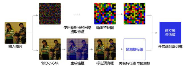
图8：YOLO-V3算法训练流程图

• 图8 左边是输入图片，上半部分所示的过程是使用卷积神经网络对图片提取特征，随着网络不断向前传播，特征图的尺寸越来越小，每个像素点会代表更加抽象的特征模式，直到输出特征图，其尺寸减小为原图的$\frac{1}{32}$。
• 图8 下半部分描述了生成候选区域的过程，首先将原图划分成多个小方块，每个小方块的大小是$32\times 32$，然后以每个小方块为中心分别生成一系列锚框，整张图片都会被锚框覆盖到。在每个锚框的基础上产生一个与之对应的预测框，根据锚框和预测框与图片上物体真实框之间的位置关系，对这些预测框进行标注。
• 将上方支路中输出的特征图与下方支路中产生的预测框标签建立关联，创建损失函数，开启端到端的训练过程。

接下来具体介绍流程中各节点的原理和代码实现。

---

产生候选区域

如何产生候选区域，是检测模型的核心设计方案。目前大多数基于卷积神经网络的模型所采用的方式大体如下：

• 按一定的规则在图片上生成一系列位置固定的锚框，将这些锚框看作是可能的候选区域。
• 对锚框是否包含目标物体进行预测，如果包含目标物体，还需要预测所包含物体的类别，以及预测框相对于锚框位置需要调整的幅度。

生成锚框

将原始图片划分成$m\times n$个区域，如下图所示，原始图片高度$H=640$, 宽度$W=480$，如果我们选择小块区域的尺寸为$32\times 32$，则$m$和$n$分别为：

$$m=\frac{640}{32}=20$$

$$n=\frac{480}{32}=15$$

如 图9 所示，将原始图像分成了20行15列小方块区域。

图9：将图片划分成多个32x32的小方块

YOLO-V3算法会在每个区域的中心，生成一系列锚框。为了展示方便，我们先在图中第十行第四列的小方块位置附近画出生成的锚框，如 图10 所示。

---

注意：

这里为了跟程序中的编号对应，最上面的行号是第0行，最左边的列号是第0列**

---

图10：在第10行第4列的小方块区域生成3个锚框

图11 展示在每个区域附近都生成3个锚框，很多锚框堆叠在一起可能不太容易看清楚，但过程跟上面类似，只是需要以每个区域的中心点为中心，分别生成3个锚框。

图11：在每个小方块区域生成3个锚框

---

生成预测框

在前面已经指出，锚框的位置都是固定好的，不可能刚好跟物体边界框重合，需要在锚框的基础上进行位置的微调以生成预测框。预测框相对于锚框会有不同的中心位置和大小，采用什么方式能得到预测框呢？我们先来考虑如何生成其中心位置坐标。

比如上面图中在第10行第4列的小方块区域中心生成的一个锚框，如绿色虚线框所示。以小方格的宽度为单位长度，

此小方块区域左上角的位置坐标是：
$$c_x=4$$
$$c_y=10$$

此锚框的区域中心坐标是：
$$center\_x=c_x+0.5=4.5$$
$$center\_y=c_y+0.5=10.5$$

可以通过下面的方式生成预测框的中心坐标：
$$b_x=c_x+\sigma (t_x)$$
$$b_y=c_y+\sigma (t_y)$$

其中$t_x$和$t_y$为实数，$\sigma (x)$是我们之前学过的Sigmoid函数，其定义如下：

$$\sigma (x)=\frac{1}{1+exp(-x)}$$

由于Sigmoid的函数值在$0\sim 1$之间，因此由上面公式计算出来的预测框的中心点总是落在第十行第四列的小区域内部。

当$t_x=t_y=0$时，$b_x=c_x+0.5$，$b_y=c_y+0.5$，预测框中心与锚框中心重合，都是小区域的中心。

锚框的大小是预先设定好的，在模型中可以当作是超参数，下图中画出的锚框尺寸是

$$p_h=350$$
$$p_w=250$$

通过下面的公式生成预测框的大小：

$$b_h=p_h{e}^{t_h}$$
$$b_w=p_w{e}^{t_w}$$

如果$t_x=t_y=0,t_h=t_w=0$，则预测框跟锚框重合。

如果给$t_x,t_y,t_h,t_w$随机赋值如下：

$$t_x=0.2,t_y=0.3,t_w=0.1,t_h=-0.12$$

则可以得到预测框的坐标是(154.98, 357.44, 276.29, 310.42)，如 图12 中蓝色框所示。

---

说明：
这里坐标采用$xywh$的格式。

---

图12：生成预测框

这里我们会问：当$t_x,t_y,t_w,t_h$取值为多少的时候，预测框能够跟真实框重合？为了回答问题，只需要将上面预测框坐标中的$b_x,b_y,b_h,b_w$设置为真实框的位置，即可求解出$t$的数值。

令：
$$\sigma (t_x^{\ast })+c_x=g{t}_x$$
$$\sigma (t_y^{\ast })+c_y=g{t}_y$$
$$p_w{e}^{t_w^{\ast }}=g{t}_h$$
$$p_h{e}^{t_h^{\ast }}=g{t}_w$$

可以求解出 $(t_x^{\ast },t_y^{\ast },t_w^{\ast },t_h^{\ast })$

如果$t$是网络预测的输出值，将$t^{\ast }$作为目标值，以他们之间的差距作为损失函数，则可以建立起一个回归问题，通过学习网络参数，使得 $t$ 足够接近 $t^{\ast }$ ，从而能够求解出预测框的位置坐标和大小。

预测框可以看作是在锚框基础上的一个微调，每个锚框会有一个跟它对应的预测框，我们需要确定上面计算式中的$t_x,t_y,t_w,t_h$，从而计算出与锚框对应的预测框的位置和形状。

---

对候选区域进行标注

每个区域可以产生3种不同形状的锚框，每个锚框都是一个可能的候选区域，对这些候选区域我们需要了解如下几件事情：

• 锚框是否包含物体，这可以看成是一个二分类问题，使用标签objectness来表示。当锚框包含了物体时，objectness=1，表示预测框属于正类；当锚框不包含物体时，设置objectness=0，表示锚框属于负类。

• 如果锚框包含了物体，那么它对应的预测框的中心位置和大小应该是多少，或者说上面计算式中的$t_x,t_y,t_w,t_h$应该是多少，使用location标签。

• 如果锚框包含了物体，那么具体类别是什么，这里使用变量label来表示其所属类别的标签。

选取任意一个锚框对它进行标注，也就是需要确定其对应的objectness, $(t_x,t_y,t_w,t_h)$和label，下面将分别讲述如何确定这三个标签的值。

---

标注锚框是否包含物体

如 图13 所示，这里一共有3个目标，以最左边的人像为例，其真实框是$(40.93,141.1,186.06,374.63)$。

图13：选出与真实框中心位于同一区域的锚框

真实框的中心点坐标是：

$$center\_x=40.93+186.06/2=133.96$$

$$center\_y=141.1+374.63/2=328.42$$

$$i=133.96/32=4.18625$$

$$j=328.42/32=10.263125$$

它落在了第10行第4列的小方块内，如图13所示。此小方块区域可以生成3个不同形状的锚框，其在图上的编号和大小分别是$A_1(116,90),A_2(156,198),A_3(373,326)$。

用这3个不同形状的锚框跟真实框计算IoU，选出IoU最大的锚框。这里为了简化计算，只考虑锚框的形状，不考虑其跟真实框中心之间的偏移，具体计算结果如 图14 所示。

图14：选出与真实框与锚框的IoU

其中跟真实框IoU最大的是锚框$A_3$，形状是$(373,326)$，将它所对应的预测框的objectness标签设置为1，其所包括的物体类别就是真实框里面的物体所属类别。

依次可以找出其他几个真实框对应的IoU最大的锚框，然后将它们的预测框的objectness标签也都设置为1。这里一共有$20\times 15\times 3=900$个锚框，只有3个预测框会被标注为正。

由于每个真实框只对应一个objectness标签为正的预测框，如果有些预测框跟真实框之间的IoU很大，但并不是最大的那个，那么直接将其objectness标签设置为0当作负样本，可能并不妥当。为了避免这种情况，YOLO-V3算法设置了一个IoU阈值iou_threshold，当预测框的objectness不为1，但是其与某个真实框的IoU大于iou_threshold时，就将其objectness标签设置为-1，不参与损失函数的计算。

所有其他的预测框，其objectness标签均设置为0，表示负类。

对于objectness=1的预测框，需要进一步确定其位置和包含物体的具体分类标签，但是对于objectness=0或者-1的预测框，则不用管他们的位置和类别。

---

标注预测框的位置坐标标签

当锚框objectness=1时，需要确定预测框位置相对于它微调的幅度，也就是锚框的位置标签。

在前面我们已经问过这样一个问题：当$t_x,t_y,t_w,t_h$取值为多少的时候，预测框能够跟真实框重合？其做法是将预测框坐标中的$b_x,b_y,b_h,b_w$设置为真实框的坐标，即可求解出$t$的数值。

令：
$$\sigma (t_x^{\ast })+c_x=g{t}_x$$
$$\sigma (t_y^{\ast })+c_y=g{t}_y$$
$$p_w{e}^{t_w^{\ast }}=g{t}_w$$
$$p_h{e}^{t_h^{\ast }}=g{t}_h$$

对于$t_x^{\ast }$和$t_y^{\ast }$，由于Sigmoid的反函数不好计算，我们直接使用$\sigma (t_x^{\ast })$和$\sigma (t_y^{\ast })$作为回归的目标。

$$d_x^{\ast }=\sigma (t_x^{\ast })=g{t}_x-c_x$$

$$d_y^{\ast }=\sigma (t_y^{\ast })=g{t}_y-c_y$$

$$t_w^{\ast }=log(\frac{g{t}_w}{p_w})$$

$$t_h^{\ast }=log(\frac{g{t}_h}{p_h})$$

如果$(t_x,t_y,t_h,t_w)$是网络预测的输出值，将$(d_x^{\ast },d_y^{\ast },t_w^{\ast },t_h^{\ast })$作为$(\sigma (t_x),\sigma (t_y),t_h,t_w)$的目标值，以它们之间的差距作为损失函数，则可以建立起一个回归问题，通过学习网络参数，使得$t$足够接近$t^{\ast }$，从而能够求解出预测框的位置。

---

标注锚框包含物体类别的标签

对于objectness=1的锚框，需要确定其具体类别。正如上面所说，objectness标注为1的锚框，会有一个真实框跟它对应，该锚框所属物体类别，即是其所对应的真实框包含的物体类别。这里使用one-hot向量来表示类别标签label。比如一共有10个分类，而真实框里面包含的物体类别是第2类，则label为$(0,1,0,0,0,0,0,0,0,0)$

对上述步骤进行总结，标注的流程如 图15 所示。

图15：标注流程示意图

通过这种方式，我们在每个小方块区域都生成了一系列的锚框作为候选区域，并且根据图片上真实物体的位置，标注出了每个候选区域对应的objectness标签、位置需要调整的幅度以及包含的物体所属的类别。位置需要调整的幅度由4个变量描述$(t_x,t_y,t_w,t_h)$，objectness标签需要用一个变量描述$obj$，描述所属类别的变量长度等于类别数C。

对于每个锚框，模型需要预测输出$(t_x,t_y,t_w,t_h,P_{obj},P_1,P_2,...,P_C)$，其中$P_{obj}$是锚框是否包含物体的概率，$P_1,P_2,...,P_C$则是锚框包含的物体属于每个类别的概率。接下来让我们一起学习如何通过卷积神经网络输出这样的预测值。

---

标注锚框的具体程序

上面描述了如何对预锚框进行标注，但读者可能仍然对里面的细节不太了解，下面将通过具体的程序完成这一步骤。

---

# 标注预测框的objectness
def get_objectness_label(img, gt_boxes, gt_labels, iou_threshold = 0.7,
                         anchors = [116, 90, 156, 198, 373, 326],
                         num_classes=7, downsample=32):
    """
    img 是输入的图像数据，形状是[N, C, H, W]
    gt_boxes，真实框，维度是[N, 50, 4]，其中50是真实框数目的上限，当图片中真实框不足50个时，不足部分的坐标全为0
              真实框坐标格式是xywh，这里使用相对值
    gt_labels，真实框所属类别，维度是[N, 50]
    iou_threshold，当预测框与真实框的iou大于iou_threshold时不将其看作是负样本
    anchors，锚框可选的尺寸
    anchor_masks，通过与anchors一起确定本层级的特征图应该选用多大尺寸的锚框
    num_classes，类别数目
    downsample，特征图相对于输入网络的图片尺寸变化的比例
    """

    img_shape = img.shape
    batchsize = img_shape[0]
    num_anchors = len(anchors) // 2
    input_h = img_shape[2]
    input_w = img_shape[3]
    # 将输入图片划分成num_rows x num_cols个小方块区域，每个小方块的边长是 downsample
    # 计算一共有多少行小方块
    num_rows = input_h // downsample
    # 计算一共有多少列小方块
    num_cols = input_w // downsample

    label_objectness = np.zeros([batchsize, num_anchors, num_rows, num_cols])
    label_classification = np.zeros([batchsize, num_anchors, num_classes, num_rows, num_cols])
    label_location = np.zeros([batchsize, num_anchors, 4, num_rows, num_cols])

    scale_location = np.ones([batchsize, num_anchors, num_rows, num_cols])

    # 对batchsize进行循环，依次处理每张图片
    for n in range(batchsize):
        # 对图片上的真实框进行循环，依次找出跟真实框形状最匹配的锚框
        for n_gt in range(len(gt_boxes[n])):
            gt = gt_boxes[n][n_gt]
            gt_cls = gt_labels[n][n_gt]
            gt_center_x = gt[0]
            gt_center_y = gt[1]
            gt_width = gt[2]
            gt_height = gt[3]
            if (gt_height < 1e-3) or (gt_height < 1e-3):
                continue
            i = int(gt_center_y * num_rows)
            j = int(gt_center_x * num_cols)
            ious = []
            for ka in range(num_anchors):
                bbox1 = [0., 0., float(gt_width), float(gt_height)]
                anchor_w = anchors[ka * 2]
                anchor_h = anchors[ka * 2 + 1]
                bbox2 = [0., 0., anchor_w/float(input_w), anchor_h/float(input_h)]
                # 计算iou
                iou = box_iou_xywh(bbox1, bbox2)
                ious.append(iou)
            ious = np.array(ious)
            inds = np.argsort(ious)
            k = inds[-1]
            label_objectness[n, k, i, j] = 1
            c = gt_cls
            label_classification[n, k, c, i, j] = 1.

            # for those prediction bbox with objectness =1, set label of location
            dx_label = gt_center_x * num_cols - j
            dy_label = gt_center_y * num_rows - i
            dw_label = np.log(gt_width * input_w / anchors[k*2])
            dh_label = np.log(gt_height * input_h / anchors[k*2 + 1])
            label_location[n, k, 0, i, j] = dx_label
            label_location[n, k, 1, i, j] = dy_label
            label_location[n, k, 2, i, j] = dw_label
            label_location[n, k, 3, i, j] = dh_label
            # scale_location用来调节不同尺寸的锚框对损失函数的贡献，作为加权系数和位置损失函数相乘
            scale_location[n, k, i, j] = 2.0 - gt_width * gt_height

    # 目前根据每张图片上所有出现过的gt box，都标注出了objectness为正的预测框，剩下的预测框则默认objectness为0
    # 对于objectness为1的预测框，标出了他们所包含的物体类别，以及位置回归的目标
    return label_objectness.astype('float32'), label_location.astype('float32'), label_classification.astype('float32'), \
             scale_location.astype('float32')

# 读取数据
reader = multithread_loader('/home/aistudio/work/insects/train', batch_size=2, mode='train')
img, gt_boxes, gt_labels, im_shape = next(reader())
# 计算出锚框对应的标签
label_objectness, label_location, label_classification, scale_location = get_objectness_label(img,
                                                                                              gt_boxes, gt_labels, 
                                                                                              iou_threshold = 0.7,
                                                                                              anchors = [116, 90, 156, 198, 373, 326],
                                                                                              num_classes=7, downsample=32)

img.shape, gt_boxes.shape, gt_labels.shape, im_shape.shape

((2, 3, 544, 544), (2, 50, 4), (2, 50), (2, 2))

label_objectness.shape, label_location.shape, label_classification.shape, scale_location.shape

((2, 3, 17, 17), (2, 3, 4, 17, 17), (2, 3, 7, 17, 17), (2, 3, 17, 17))

上面的程序实现了对锚框进行标注，对于每个真实框，选出了与它形状最匹配的锚框，将其objectness标注为1，并且将$[d_x^{\ast },d_y^{\ast },t_h^{\ast },t_w^{\ast }]$作为正样本位置的标签，真实框包含的物体类别作为锚框的类别。而其余的锚框，objectness将被标注为0，无需标注出位置和类别的标签。

• 注意：这里还遗留一个小问题，前面我们说了对于与真实框IoU较大的那些锚框，需要将其objectness标注为-1，不参与损失函数的计算。我们先将这个问题放一放，等到后面建立损失函数的时候再补上。

---

卷积神经网络提取特征

在上一节图像分类的课程中，我们已经学习过了通过卷积神经网络提取图像特征。通过连续使用多层卷积和池化等操作，能得到语义含义更加丰富的特征图。在检测问题中，也使用卷积神经网络逐层提取图像特征，通过最终的输出特征图来表征物体位置和类别等信息。

YOLO-V3算法使用的骨干网络是Darknet53。Darknet53网络的具体结构如 图16 所示，在ImageNet图像分类任务上取得了很好的成绩。在检测任务中，将图中C0后面的平均池化、全连接层和Softmax去掉，保留从输入到C0部分的网络结构，作为检测模型的基础网络结构，也称为骨干网络。YOLO-V3模型会在骨干网络的基础上，再添加检测相关的网络模块。

图16：Darknet53网络结构

下面的程序是Darknet53骨干网络的实现代码，这里将上图中C0、C1、C2所表示的输出数据取出，并查看它们的形状分别是，$C0[1,1024,20,20]$，$C1[1,512,40,40]$，$C2[1,256,80,80]$。

• 名词解释：特征图的步幅(stride)

在提取特征的过程中通常会使用步幅大于1的卷积或者池化，导致后面的特征图尺寸越来越小，特征图的步幅等于输入图片尺寸除以特征图尺寸。例如C0的尺寸是$20\times 20$，原图尺寸是$640\times 640$，则C0的步幅是$\frac{640}{20}=32$。同理，C1的步幅是16，C2的步幅是8。

---

import paddle.fluid as fluid
from paddle.fluid.param_attr import ParamAttr
from paddle.fluid.regularizer import L2Decay

from paddle.fluid.dygraph.nn import Conv2D, BatchNorm
from paddle.fluid.dygraph.base import to_variable

# YOLO-V3骨干网络结构Darknet53的实现代码

class ConvBNLayer(fluid.dygraph.Layer):
    """
    卷积 + 批归一化，BN层之后激活函数默认用leaky_relu
    """
    def __init__(self,
                 ch_in,
                 ch_out,
                 filter_size=3,
                 stride=1,
                 groups=1,
                 padding=0,
                 act="leaky",
                 is_test=True):
        super(ConvBNLayer, self).__init__()

        self.conv = Conv2D(
            num_channels=ch_in,
            num_filters=ch_out,
            filter_size=filter_size,
            stride=stride,
            padding=padding,
            groups=groups,
            param_attr=ParamAttr(
                initializer=fluid.initializer.Normal(0., 0.02)),
            bias_attr=False,
            act=None)

        self.batch_norm = BatchNorm(
            num_channels=ch_out,
            is_test=is_test,
            param_attr=ParamAttr(
                initializer=fluid.initializer.Normal(0., 0.02),
                regularizer=L2Decay(0.)),
            bias_attr=ParamAttr(
                initializer=fluid.initializer.Constant(0.0),
                regularizer=L2Decay(0.)))
        self.act = act

    def forward(self, inputs):
        out = self.conv(inputs)
        out = self.batch_norm(out)
        if self.act == 'leaky':
            out = fluid.layers.leaky_relu(x=out, alpha=0.1)
        return out

class DownSample(fluid.dygraph.Layer):
    """
    下采样，图片尺寸减半，具体实现方式是使用stirde=2的卷积
    """
    def __init__(self,
                 ch_in,
                 ch_out,
                 filter_size=3,
                 stride=2,
                 padding=1,
                 is_test=True):

        super(DownSample, self).__init__()

        self.conv_bn_layer = ConvBNLayer(
            ch_in=ch_in,
            ch_out=ch_out,
            filter_size=filter_size,
            stride=stride,
            padding=padding,
            is_test=is_test)
        self.ch_out = ch_out
    def forward(self, inputs):
        out = self.conv_bn_layer(inputs)
        return out

class BasicBlock(fluid.dygraph.Layer):
    """
    基本残差块的定义，输入x经过两层卷积，然后接第二层卷积的输出和输入x相加
    """
    def __init__(self, ch_in, ch_out, is_test=True):
        super(BasicBlock, self).__init__()

        self.conv1 = ConvBNLayer(
            ch_in=ch_in,
            ch_out=ch_out,
            filter_size=1,
            stride=1,
            padding=0,
            is_test=is_test
            )
        self.conv2 = ConvBNLayer(
            ch_in=ch_out,
            ch_out=ch_out*2,
            filter_size=3,
            stride=1,
            padding=1,
            is_test=is_test
            )
    def forward(self, inputs):
        conv1 = self.conv1(inputs)
        conv2 = self.conv2(conv1)
        out = fluid.layers.elementwise_add(x=inputs, y=conv2, act=None)
        return out

class LayerWarp(fluid.dygraph.Layer):
    """
    添加多层残差块，组成Darknet53网络的一个层级
    """
    def __init__(self, ch_in, ch_out, count, is_test=True):
        super(LayerWarp,self).__init__()

        self.basicblock0 = BasicBlock(ch_in,
            ch_out,
            is_test=is_test)
        self.res_out_list = []
        for i in range(1, count):
            res_out = self.add_sublayer("basic_block_%d" % (i), #使用add_sublayer添加子层
                BasicBlock(ch_out*2,
                    ch_out,
                    is_test=is_test))
            self.res_out_list.append(res_out)

    def forward(self,inputs):
        y = self.basicblock0(inputs)
        for basic_block_i in self.res_out_list:
            y = basic_block_i(y)
        return y

DarkNet_cfg = {
     53: ([1, 2, 8, 8, 4])}

class DarkNet53_conv_body(fluid.dygraph.Layer):
    def __init__(self,
                 
                 is_test=True):
        super(DarkNet53_conv_body, self).__init__()
        self.stages = DarkNet_cfg[53]
        self.stages = self.stages[0:5]

        # 第一层卷积
        self.conv0 = ConvBNLayer(
            ch_in=3,
            ch_out=32,
            filter_size=3,
            stride=1,
            padding=1,
            is_test=is_test)

        # 下采样，使用stride=2的卷积来实现
        self.downsample0 = DownSample(
            ch_in=32,
            ch_out=32 * 2,
            is_test=is_test)

        # 添加各个层级的实现
        self.darknet53_conv_block_list = []
        self.downsample_list = []
        for i, stage in enumerate(self.stages):
            conv_block = self.add_sublayer(
                "stage_%d" % (i),
                LayerWarp(32*(2**(i+1)),
                32*(2**i),
                stage,
                is_test=is_test))
            self.darknet53_conv_block_list.append(conv_block)
        # 两个层级之间使用DownSample将尺寸减半
        for i in range(len(self.stages) - 1):
            downsample = self.add_sublayer(
                "stage_%d_downsample" % i,
                DownSample(ch_in=32*(2**(i+1)),
                    ch_out=32*(2**(i+2)),
                    is_test=is_test))
            self.downsample_list.append(downsample)

    def forward(self,inputs):
        out = self.conv0(inputs)
        #print("conv1:",out.numpy())
        out = self.downsample0(out)
        #print("dy:",out.numpy())
        blocks = []
        for i, conv_block_i in enumerate(self.darknet53_conv_block_list): #依次将各个层级作用在输入上面
            out = conv_block_i(out)
            blocks.append(out)
            if i < len(self.stages) - 1:
                out = self.downsample_list[i](out)
        return blocks[-1:-4:-1] # 将C0, C1, C2作为返回值

# 查看Darknet53网络输出特征图
import numpy as np
with fluid.dygraph.guard():
    backbone = DarkNet53_conv_body(is_test=False)
    x = np.random.randn(1, 3, 640, 640).astype('float32')
    x = to_variable(x)
    C0, C1, C2 = backbone(x)
    print(C0.shape, C1.shape, C2.shape)

[1, 1024, 20, 20] [1, 512, 40, 40] [1, 256, 80, 80]

上面这段示例代码，指定输入数据的形状是$(1,3,640,640)$，则3个层级的输出特征图的形状分别是$C0(1,1024,20,20)$，$C1(1,1024,40,40)$和$C2(1,1024,80,80)$。

根据输出特征图计算预测框位置和类别

YOLO-V3中对每个预测框计算逻辑如下：

• 预测框是否包含物体。也可理解为objectness=1的概率是多少，可以用网络输出一个实数$x$，可以用$Sigmoid(x)$表示objectness为正的概率$P_{obj}$

• 预测物体位置和形状。物体位置和形状$t_x,t_y,t_w,t_h$可以用网络输出4个实数来表示$t_x,t_y,t_w,t_h$

• 预测物体类别。预测图像中物体的具体类别是什么，或者说其属于每个类别的概率分别是多少。总的类别数为C，需要预测物体属于每个类别的概率$(P_1,P_2,...,P_C)$，可以用网络输出C个实数$(x_1,x_2,...,x_C)$，对每个实数分别求Sigmoid函数，让$P_i=Sigmoid(x_i)$，则可以表示出物体属于每个类别的概率。

对于一个预测框，网络需要输出$(5+C)$个实数来表征它是否包含物体、位置和形状尺寸以及属于每个类别的概率。

由于我们在每个小方块区域都生成了K个预测框，则所有预测框一共需要网络输出的预测值数目是：

$$[K(5+C)]\times m\times n$$

还有更重要的一点是网络输出必须要能区分出小方块区域的位置来，不能直接将特征图连接一个输出大小为$[K(5+C)]\times m\times n$的全连接层。

---

建立输出特征图与预测框之间的关联

现在观察特征图，经过多次卷积核池化之后，其步幅stride=32，$640\times 480$大小的输入图片变成了$20\times 15$的特征图；而小方块区域的数目正好是$20\times 15$，也就是说可以让特征图上每个像素点分别跟原图上一个小方块区域对应。这也是为什么我们最开始将小方块区域的尺寸设置为32的原因，这样可以巧妙的将小方块区域跟特征图上的像素点对应起来，解决了空间位置的对应关系。

图17：特征图C0与小方块区域形状对比

下面需要将像素点$(i,j)$与第i行第j列的小方块区域所需要的预测值关联起来，每个小方块区域产生K个预测框，每个预测框需要$(5+C)$个实数预测值，则每个像素点相对应的要有$K(5+C)$个实数。为了解决这一问题，对特征图进行多次卷积，并将最终的输出通道数设置为$K(5+C)$，即可将生成的特征图与每个预测框所需要的预测值巧妙的对应起来。

骨干网络的输出特征图是C0，下面的程序是对C0进行多次卷积以得到跟预测框相关的特征图P0。

# 从骨干网络输出特征图C0得到跟预测相关的特征图P0
class YoloDetectionBlock(fluid.dygraph.Layer):
    # define YOLO-V3 detection head
    # 使用多层卷积和BN提取特征
    def __init__(self,ch_in,ch_out,is_test=True):
        super(YoloDetectionBlock, self).__init__()

        assert ch_out % 2 == 0, \
            "channel {} cannot be divided by 2".format(ch_out)

        self.conv0 = ConvBNLayer(
            ch_in=ch_in,
            ch_out=ch_out,
            filter_size=1,
            stride=1,
            padding=0,
            is_test=is_test
            )
        self.conv1 = ConvBNLayer(
            ch_in=ch_out,
            ch_out=ch_out*2,
            filter_size=3,
            stride=1,
            padding=1,
            is_test=is_test
            )
        self.conv2 = ConvBNLayer(
            ch_in=ch_out*2,
            ch_out=ch_out,
            filter_size=1,
            stride=1,
            padding=0,
            is_test=is_test
            )
        self.conv3 = ConvBNLayer(
            ch_in=ch_out,
            ch_out=ch_out*2,
            filter_size=3,
            stride=1,
            padding=1,
            is_test=is_test
            )
        self.route = ConvBNLayer(
            ch_in=ch_out*2,
            ch_out=ch_out,
            filter_size=1,
            stride=1,
            padding=0,
            is_test=is_test
            )
        self.tip = ConvBNLayer(
            ch_in=ch_out,
            ch_out=ch_out*2,
            filter_size=3,
            stride=1,
            padding=1,
            is_test=is_test
            )
    def forward(self, inputs):
        out = self.conv0(inputs)
        out = self.conv1(out)
        out = self.conv2(out)
        out = self.conv3(out)
        route = self.route(out)
        tip = self.tip(route)
        return route, tip

NUM_ANCHORS = 3
NUM_CLASSES = 7
num_filters=NUM_ANCHORS * (NUM_CLASSES + 5)
with fluid.dygraph.guard():
    backbone = DarkNet53_conv_body(is_test=False)
    detection = YoloDetectionBlock(ch_in=1024, ch_out=512, is_test=False)
    conv2d_pred = Conv2D(num_channels=1024, num_filters=num_filters,  filter_size=1)
    
    x = np.random.randn(1, 3, 640, 640).astype('float32')
    x = to_variable(x)
    C0, C1, C2 = backbone(x)
    route, tip = detection(C0)
    P0 = conv2d_pred(tip)
    
    print(P0.shape)

[1, 36, 20, 20]

如上面的代码所示，可以由特征图C0生成特征图P0，P0的形状是$[1,36,20,20]$。每个小方块区域生成的锚框或者预测框的数量是3，物体类别数目是7，每个区域需要的预测值个数是$3\times (5+7)=36$，正好等于P0的输出通道数。

图18：特征图P0与候选区域的关联

将$P0[t,0:12,i,j]$与输入的第t张图片上小方块区域$(i,j)$第1个预测框所需要的12个预测值对应，$P0[t,12:24,i,j]$与输入的第t张图片上小方块区域$(i,j)$第2个预测框所需要的12个预测值对应，$P0[t,24:36,i,j]$与输入的第t张图片上小方块区域$(i,j)$第3个预测框所需要的12个预测值对应。

$P0[t,0:4,i,j]$与输入的第t张图片上小方块区域$(i,j)$第1个预测框的位置对应，$P0[t,4,i,j]$与输入的第t张图片上小方块区域$(i,j)$第1个预测框的objectness对应，$P0[t,5:12,i,j]$与输入的第t张图片上小方块区域$(i,j)$第1个预测框的类别对应。

如 图18 所示，通过这种方式可以巧妙的将网络输出特征图，与每个小方块区域生成的预测框对应起来了。

---

计算预测框是否包含物体的概率

根据前面的分析，$P0[t,4,i,j]$与输入的第t张图片上小方块区域$(i,j)$第1个预测框的objectness对应，$P0[t,4+12,i,j]$与第2个预测框的objectness对应，…，则可以使用下面的程序将objectness相关的预测取出，并使用fluid.layers.sigmoid计算输出概率。

NUM_ANCHORS = 3
NUM_CLASSES = 7
num_filters=NUM_ANCHORS * (NUM_CLASSES + 5)
with fluid.dygraph.guard():
    backbone = DarkNet53_conv_body(is_test=False)
    detection = YoloDetectionBlock(ch_in=1024, ch_out=512, is_test=False)
    conv2d_pred = Conv2D(num_channels=1024, num_filters=num_filters,  filter_size=1)
    
    x = np.random.randn(1, 3, 640, 640).astype('float32')
    x = to_variable(x)
    C0, C1, C2 = backbone(x)
    route, tip = detection(C0)
    P0 = conv2d_pred(tip)
    
    reshaped_p0 = fluid.layers.reshape(P0, [-1, NUM_ANCHORS, NUM_CLASSES + 5, P0.shape[2], P0.shape[3]])
    pred_objectness = reshaped_p0[:, :, 4, :, :]
    pred_objectness_probability = fluid.layers.sigmoid(pred_objectness)
    print(pred_objectness.shape, pred_objectness_probability.shape)

[1, 3, 20, 20] [1, 3, 20, 20]

上面的输出程序显示，预测框是否包含物体的概率pred_objectness_probability，其数据形状是$[1, 3, 20, 20] $，与我们上面提到的预测框个数一致，数据大小在0～1之间，表示预测框为正样本的概率。

计算预测框位置坐标

$P0[t,0:4,i,j]$与输入的第$t$张图片上小方块区域$(i,j)$第1个预测框的位置对应，$P0[t,12:16,i,j]$与第2个预测框的位置对应，…，使用下面的程序可以从$P0$中取出跟预测框位置相关的预测值。

NUM_ANCHORS = 3
NUM_CLASSES = 7
num_filters=NUM_ANCHORS * (NUM_CLASSES + 5)
with fluid.dygraph.guard():
    backbone = DarkNet53_conv_body(is_test=False)
    detection = YoloDetectionBlock(ch_in=1024, ch_out=512, is_test=False)
    conv2d_pred = Conv2D(num_channels=1024, num_filters=num_filters,  filter_size=1)
    
    x = np.random.randn(1, 3, 640, 640).astype('float32')
    x = to_variable(x)
    C0, C1, C2 = backbone(x)
    route, tip = detection(C0)
    P0 = conv2d_pred(tip)
    

    reshaped_p0 = fluid.layers.reshape(P0, [-1, NUM_ANCHORS, NUM_CLASSES + 5, P0.shape[2], P0.shape[3]])
    pred_objectness = reshaped_p0[:, :, 4, :, :]
    pred_objectness_probability = fluid.layers.sigmoid(pred_objectness)

    pred_location = reshaped_p0[:, :, 0:4, :, :]
    print(pred_location.shape)
    

[1, 3, 4, 20, 20]

网络输出值是$(t_x,t_y,t_h,t_w)$，还需要将其转化为$(x_1,y_1,x_2,y_2)$这种形式的坐标表示。使用飞桨fluid.layers.yolo_box API可以直接计算出结果，但为了给读者更清楚的展示算法的实现过程，我们使用Numpy来实现这一过程。

# 定义Sigmoid函数
def sigmoid(x):
    return 1./(1.0 + np.exp(-x))

# 将网络特征图输出的[tx, ty, th, tw]转化成预测框的坐标[x1, y1, x2, y2]
def get_yolo_box_xxyy(pred, anchors, num_classes, downsample):
    """
    pred是网络输出特征图转化成的numpy.ndarray
    anchors 是一个list。表示锚框的大小，
                例如 anchors = [116, 90, 156, 198, 373, 326]，表示有三个锚框，
                第一个锚框大小[w, h]是[116, 90]，第二个锚框大小是[156, 198]，第三个锚框大小是[373, 326]
    """
    batchsize = pred.shape[0]
    num_rows = pred.shape[-2]
    num_cols = pred.shape[-1]

    input_h = num_rows * downsample
    input_w = num_cols * downsample

    num_anchors = len(anchors) // 2

    # pred的形状是[N, C, H, W]，其中C = NUM_ANCHORS * (5 + NUM_CLASSES)
    # 对pred进行reshape
    pred = pred.reshape([-1, num_anchors, 5+num_classes, num_rows, num_cols])
    pred_location = pred[:, :, 0:4, :, :]
    pred_location = np.transpose(pred_location, (0,3,4,1,2))
    anchors_this = []
    for ind in range(num_anchors):
        anchors_this.append([anchors[ind*2], anchors[ind*2+1]])
    anchors_this = np.array(anchors_this).astype('float32')
    
    # 最终输出数据保存在pred_box中，其形状是[N, H, W, NUM_ANCHORS, 4]，
    # 其中最后一个维度4代表位置的4个坐标
    pred_box = np.zeros(pred_location.shape)
    for n in range(batchsize):
        for i in range(num_rows):
            for j in range(num_cols):
                for k in range(num_anchors):
                    pred_box[n, i, j, k, 0] = j
                    pred_box[n, i, j, k, 1] = i
                    pred_box[n, i, j, k, 2] = anchors_this[k][0]
                    pred_box[n, i, j, k, 3] = anchors_this[k][1]

    # 这里使用相对坐标，pred_box的输出元素数值在0.~1.0之间
    pred_box[:, :, :, :, 0] = (sigmoid(pred_location[:, :, :, :, 0]) + pred_box[:, :, :, :, 0]) / num_cols
    pred_box[:, :, :, :, 1] = (sigmoid(pred_location[:, :, :, :, 1]) + pred_box[:, :, :, :, 1]) / num_rows
    pred_box[:, :, :, :, 2] = np.exp(pred_location[:, :, :, :, 2]) * pred_box[:, :, :, :, 2] / input_w
    pred_box[:, :, :, :, 3] = np.exp(pred_location[:, :, :, :, 3]) * pred_box[:, :, :, :, 3] / input_h

    # 将坐标从xywh转化成xyxy
    pred_box[:, :, :, :, 0] = pred_box[:, :, :, :, 0] - pred_box[:, :, :, :, 2] / 2.
    pred_box[:, :, :, :, 1] = pred_box[:, :, :, :, 1] - pred_box[:, :, :, :, 3] / 2.
    pred_box[:, :, :, :, 2] = pred_box[:, :, :, :, 0] + pred_box[:, :, :, :, 2]
    pred_box[:, :, :, :, 3] = pred_box[:, :, :, :, 1] + pred_box[:, :, :, :, 3]

    pred_box = np.clip(pred_box, 0., 1.0)

    return pred_box

通过调用上面定义的get_yolo_box_xxyy函数，可以从$P0$计算出预测框坐标来，具体程序如下：

NUM_ANCHORS = 3
NUM_CLASSES = 7
num_filters=NUM_ANCHORS * (NUM_CLASSES + 5)
with fluid.dygraph.guard():
    backbone = DarkNet53_conv_body(is_test=False)
    detection = YoloDetectionBlock(ch_in=1024, ch_out=512, is_test=False)
    conv2d_pred = Conv2D(num_channels=1024, num_filters=num_filters,  filter_size=1)
    
    x = np.random.randn(1, 3, 640, 640).astype('float32')
    x = to_variable(x)
    C0, C1, C2 = backbone(x)
    route, tip = detection(C0)
    P0 = conv2d_pred(tip)
    
    reshaped_p0 = fluid.layers.reshape(P0, [-1, NUM_ANCHORS, NUM_CLASSES + 5, P0.shape[2], P0.shape[3]])
    pred_objectness = reshaped_p0[:, :, 4, :, :]
    pred_objectness_probability = fluid.layers.sigmoid(pred_objectness)

    pred_location = reshaped_p0[:, :, 0:4, :, :]
    
    # anchors包含了预先设定好的锚框尺寸
    anchors = [116, 90, 156, 198, 373, 326]
    # downsample是特征图P0的步幅
    pred_boxes = get_yolo_box_xxyy(P0.numpy(), anchors, num_classes=7, downsample=32) # 由输出特征图P0计算预测框位置坐标
    print(pred_boxes.shape)

(1, 20, 20, 3, 4)

上面程序计算出来的pred_boxes的形状是$[N,H,W,num\_anchors,4]$，坐标格式是$[x_1,y_1,x_2,y_2]$，数值在0~1之间，表示相对坐标。

计算物体属于每个类别概率

$P0[t,5:12,i,j]$与输入的第$t$张图片上小方块区域$(i,j)$第1个预测框包含物体的类别对应，$P0[t,17:24,i,j]$与第2个预测框的类别对应，…，使用下面的程序可以从$P0$中取出那些跟预测框类别相关的预测值。

NUM_ANCHORS = 3
NUM_CLASSES = 7
num_filters=NUM_ANCHORS * (NUM_CLASSES + 5)
with fluid.dygraph.guard():
    backbone = DarkNet53_conv_body(is_test=False)
    detection = YoloDetectionBlock(ch_in=1024, ch_out=512, is_test=False)
    conv2d_pred = Conv2D(num_channels=1024, num_filters=num_filters,  filter_size=1)
    
    x = np.random.randn(1, 3, 640, 640).astype('float32')
    x = to_variable(x)
    C0, C1, C2 = backbone(x)
    route, tip = detection(C0)
    P0 = conv2d_pred(tip)
    
    reshaped_p0 = fluid.layers.reshape(P0, [-1, NUM_ANCHORS, NUM_CLASSES + 5, P0.shape[2], P0.shape[3]])
    # 取出与objectness相关的预测值
    pred_objectness = reshaped_p0[:, :, 4, :, :]
    pred_objectness_probability = fluid.layers.sigmoid(pred_objectness)
    # 取出与位置相关的预测值
    pred_location = reshaped_p0[:, :, 0:4, :, :]
    # 取出与类别相关的预测值
    pred_classification = reshaped_p0[:, :, 5:5+NUM_CLASSES, :, :]
    pred_classification_probability = fluid.layers.sigmoid(pred_classification)
    print(pred_classification.shape)

[1, 3, 7, 20, 20]

上面的程序通过$P0$计算出了预测框包含的物体所属类别的概率，pred_classification_probability的形状是$[1,3,7,20,20]$，数值在0~1之间。

损失函数

上面从概念上将输出特征图上的像素点与预测框关联起来了，那么要对神经网络进行求解，还必须从数学上将网络输出和预测框关联起来，也就是要建立起损失函数跟网络输出之间的关系。下面讨论如何建立起YOLO-V3的损失函数。

对于每个预测框，YOLO-V3模型会建立三种类型的损失函数：

• 表征是否包含目标物体的损失函数，通过pred_objectness和label_objectness计算。

    loss_obj = fluid.layers.sigmoid_cross_entropy_with_logits(pred_objectness, label_objectness)
  

• 表征物体位置的损失函数，通过pred_location和label_location计算。

    pred_location_x = pred_location[:, :, 0, :, :]
    pred_location_y = pred_location[:, :, 1, :, :]
    pred_location_w = pred_location[:, :, 2, :, :]
    pred_location_h = pred_location[:, :, 3, :, :]
    loss_location_x = fluid.layers.sigmoid_cross_entropy_with_logits(pred_location_x, label_location_x)
    loss_location_y = fluid.layers.sigmoid_cross_entropy_with_logits(pred_location_y, label_location_y)
    loss_location_w = fluid.layers.abs(pred_location_w - label_location_w)
    loss_location_h = fluid.layers.abs(pred_location_h - label_location_h)
    loss_location = loss_location_x + loss_location_y + loss_location_w + loss_location_h
  

• 表征物体类别的损失函数，通过pred_classification和label_classification计算。

    loss_obj = fluid.layers.sigmoid_cross_entropy_with_logits(pred_classification, label_classification)
  

我们已经知道怎么计算这些预测值和标签了，但是遗留了一个小问题，就是没有标注出哪些锚框的objectness为-1。为了完成这一步，我们需要计算出所有预测框跟真实框之间的IoU，然后把那些IoU大于阈值的真实框挑选出来。实现代码如下：

# 挑选出跟真实框IoU大于阈值的预测框
def get_iou_above_thresh_inds(pred_box, gt_boxes, iou_threshold):
    batchsize = pred_box.shape[0]
    num_rows = pred_box.shape[1]
    num_cols = pred_box.shape[2]
    num_anchors = pred_box.shape[3]
    ret_inds = np.zeros([batchsize, num_rows, num_cols, num_anchors])
    for i in range(batchsize):
        pred_box_i = pred_box[i]
        gt_boxes_i = gt_boxes[i]
        for k in range(len(gt_boxes_i)): #gt in gt_boxes_i:
            gt = gt_boxes_i[k]
            gtx_min = gt[0] - gt[2] / 2.
            gty_min = gt[1] - gt[3] / 2.
            gtx_max = gt[0] + gt[2] / 2.
            gty_max = gt[1] + gt[3] / 2.
            if (gtx_max - gtx_min < 1e-3) or (gty_max - gty_min < 1e-3):
                continue
            x1 = np.maximum(pred_box_i[:, :, :, 0], gtx_min)
            y1 = np.maximum(pred_box_i[:, :, :, 1], gty_min)
            x2 = np.minimum(pred_box_i[:, :, :, 2], gtx_max)
            y2 = np.minimum(pred_box_i[:, :, :, 3], gty_max)
            intersection = np.maximum(x2 - x1, 0.) * np.maximum(y2 - y1, 0.)
            s1 = (gty_max - gty_min) * (gtx_max - gtx_min)
            s2 = (pred_box_i[:, :, :, 2] - pred_box_i[:, :, :, 0]) * (pred_box_i[:, :, :, 3] - pred_box_i[:, :, :, 1])
            union = s2 + s1 - intersection
            iou = intersection / union
            above_inds = np.where(iou > iou_threshold)
            ret_inds[i][above_inds] = 1
    ret_inds = np.transpose(ret_inds, (0,3,1,2))
    return ret_inds.astype('bool')

上面的函数可以得到哪些锚框的objectness需要被标注为-1，通过下面的程序，对label_objectness进行处理，将IoU大于阈值，但又不是正样本的锚框标注为-1。

def label_objectness_ignore(label_objectness, iou_above_thresh_indices):
    # 注意：这里不能简单的使用 label_objectness[iou_above_thresh_indices] = -1，
    #         这样可能会造成label_objectness为1的点被设置为-1了
    #         只有将那些被标注为0，且与真实框IoU超过阈值的预测框才被标注为-1
    negative_indices = (label_objectness < 0.5)
    ignore_indices = negative_indices * iou_above_thresh_indices
    label_objectness[ignore_indices] = -1
    return label_objectness

下面通过调用这两个函数，实现如何将部分预测框的label_objectness设置为-1。

# 读取数据
reader = multithread_loader('/home/aistudio/work/insects/train', batch_size=2, mode='train')
img, gt_boxes, gt_labels, im_shape = next(reader())
# 计算出锚框对应的标签
label_objectness, label_location, label_classification, scale_location = get_objectness_label(img,
                                                                                              gt_boxes, gt_labels, 
                                                                                              iou_threshold = 0.7,
                                                                                              anchors = [116, 90, 156, 198, 373, 326],
                                                                                              num_classes=7, downsample=32)
NUM_ANCHORS = 3
NUM_CLASSES = 7
num_filters=NUM_ANCHORS * (NUM_CLASSES + 5)
with fluid.dygraph.guard():
    backbone = DarkNet53_conv_body(is_test=False)
    detection = YoloDetectionBlock(ch_in=1024, ch_out=512, is_test=False)
    conv2d_pred = Conv2D(num_channels=1024, num_filters=num_filters,  filter_size=1)
    
    
    x = to_variable(img)
    C0, C1, C2 = backbone(x)
    route, tip = detection(C0)
    P0 = conv2d_pred(tip)
    
    # anchors包含了预先设定好的锚框尺寸
    anchors = [116, 90, 156, 198, 373, 326]
    # downsample是特征图P0的步幅
    pred_boxes = get_yolo_box_xxyy(P0.numpy(), anchors, num_classes=7, downsample=32)
    iou_above_thresh_indices = get_iou_above_thresh_inds(pred_boxes, gt_boxes, iou_threshold=0.7)
    label_objectness = label_objectness_ignore(label_objectness, iou_above_thresh_indices)
    print(label_objectness.shape)

(2, 3, 15, 15)

使用这种方式，就可以将那些没有被标注为正样本，但又与真实框IoU比较大的样本objectness标签设置为-1了，不计算其对任何一种损失函数的贡献。计算总的损失函数的代码如下：

def get_loss(output, label_objectness, label_location, label_classification, scales, num_anchors=3, num_classes=7):
    # 将output从[N, C, H, W]变形为[N, NUM_ANCHORS, NUM_CLASSES + 5, H, W]
    reshaped_output = fluid.layers.reshape(output, [-1, num_anchors, num_classes + 5, output.shape[2], output.shape[3]])

    # 从output中取出跟objectness相关的预测值
    pred_objectness = reshaped_output[:, :, 4, :, :]
    loss_objectness = fluid.layers.sigmoid_cross_entropy_with_logits(pred_objectness, label_objectness, ignore_index=-1)
    ## 对第1，2，3维求和
    #loss_objectness = fluid.layers.reduce_sum(loss_objectness, dim=[1,2,3], keep_dim=False)

    # pos_samples 只有在正样本的地方取值为1.，其它地方取值全为0.
    pos_objectness = label_objectness > 0
    pos_samples = fluid.layers.cast(pos_objectness, 'float32')
    pos_samples.stop_gradient=True

    #从output中取出所有跟位置相关的预测值
    tx = reshaped_output[:, :, 0, :, :]
    ty = reshaped_output[:, :, 1, :, :]
    tw = reshaped_output[:, :, 2, :, :]
    th = reshaped_output[:, :, 3, :, :]

    # 从label_location中取出各个位置坐标的标签
    dx_label = label_location[:, :, 0, :, :]
    dy_label = label_location[:, :, 1, :, :]
    tw_label = label_location[:, :, 2, :, :]
    th_label = label_location[:, :, 3, :, :]
    # 构建损失函数
    loss_location_x = fluid.layers.sigmoid_cross_entropy_with_logits(tx, dx_label)
    loss_location_y = fluid.layers.sigmoid_cross_entropy_with_logits(ty, dy_label)
    loss_location_w = fluid.layers.abs(tw - tw_label)
    loss_location_h = fluid.layers.abs(th - th_label)

    # 计算总的位置损失函数
    loss_location = loss_location_x + loss_location_y + loss_location_h + loss_location_w

    # 乘以scales
    loss_location = loss_location * scales
    # 只计算正样本的位置损失函数
    loss_location = loss_location * pos_samples

    #从ooutput取出所有跟物体类别相关的像素点
    pred_classification = reshaped_output[:, :, 5:5+num_classes, :, :]
    # 计算分类相关的损失函数
    loss_classification = fluid.layers.sigmoid_cross_entropy_with_logits(pred_classification, label_classification)
    # 将第2维求和
    loss_classification = fluid.layers.reduce_sum(loss_classification, dim=2, keep_dim=False)
    # 只计算objectness为正的样本的分类损失函数
    loss_classification = loss_classification * pos_samples
    total_loss = loss_objectness + loss_location + loss_classification
    # 对所有预测框的loss进行求和
    total_loss = fluid.layers.reduce_sum(total_loss, dim=[1,2,3], keep_dim=False)
    # 对所有样本求平均
    total_loss = fluid.layers.reduce_mean(total_loss)

    return total_loss

# 计算损失函数

# 读取数据
reader = multithread_loader('/home/aistudio/work/insects/train', batch_size=2, mode='train')
img, gt_boxes, gt_labels, im_shape = next(reader())
# 计算出锚框对应的标签
label_objectness, label_location, label_classification, scale_location = get_objectness_label(img,
                                                                                              gt_boxes, gt_labels, 
                                                                                              iou_threshold = 0.7,
                                                                                              anchors = [116, 90, 156, 198, 373, 326],
                                                                                              num_classes=7, downsample=32)
NUM_ANCHORS = 3
NUM_CLASSES = 7
num_filters=NUM_ANCHORS * (NUM_CLASSES + 5)
with fluid.dygraph.guard():
    backbone = DarkNet53_conv_body(is_test=False)
    detection = YoloDetectionBlock(ch_in=1024, ch_out=512, is_test=False)
    conv2d_pred = Conv2D(num_channels=1024, num_filters=num_filters,  filter_size=1)
    
    x = to_variable(img)
    C0, C1, C2 = backbone(x)
    route, tip = detection(C0)
    P0 = conv2d_pred(tip)
    # anchors包含了预先设定好的锚框尺寸
    anchors = [116, 90, 156, 198, 373, 326]
    # downsample是特征图P0的步幅
    pred_boxes = get_yolo_box_xxyy(P0.numpy(), anchors, num_classes=7, downsample=32)
    iou_above_thresh_indices = get_iou_above_thresh_inds(pred_boxes, gt_boxes, iou_threshold=0.7)
    label_objectness = label_objectness_ignore(label_objectness, iou_above_thresh_indices)
    
    label_objectness = to_variable(label_objectness)
    label_location = to_variable(label_location)
    label_classification = to_variable(label_classification)
    scales = to_variable(scale_location)
    label_objectness.stop_gradient=True
    label_location.stop_gradient=True
    label_classification.stop_gradient=True
    scales.stop_gradient=True
    
    total_loss = get_loss(P0, label_objectness, label_location, label_classification, scales,
                              num_anchors=NUM_ANCHORS, num_classes=NUM_CLASSES)
    total_loss_data = total_loss.numpy()
    print(total_loss_data)
    

[324.15128]

上面的程序计算出了总的损失函数，看到这里，读者已经了解到了YOLO-V3算法的大部分内容，包括如何生成锚框、给锚框打上标签、通过卷积神经网络提取特征、将输出特征图跟预测框相关联、建立起损失函数。

---